Last updated: 2025-05-30

Checks: 7 0

Knit directory: prs/

This reproducible R Markdown analysis was created with workflowr (version 1.7.1). The Checks tab describes the reproducibility checks that were applied when the results were created. The Past versions tab lists the development history.

R Markdown file: up-to-date

Great! Since the R Markdown file has been committed to the Git repository, you know the exact version of the code that produced these results.

Environment: empty

Great job! The global environment was empty. Objects defined in the global environment can affect the analysis in your R Markdown file in unknown ways. For reproduciblity it’s best to always run the code in an empty environment.

Seed: set.seed(20250417)

The command set.seed(20250417) was run prior to running the code in the R Markdown file. Setting a seed ensures that any results that rely on randomness, e.g. subsampling or permutations, are reproducible.

Session information: recorded

Great job! Recording the operating system, R version, and package versions is critical for reproducibility.

Cache: none

Nice! There were no cached chunks for this analysis, so you can be confident that you successfully produced the results during this run.

File paths: relative

Great job! Using relative paths to the files within your workflowr project makes it easier to run your code on other machines.

Repository version: dd36c42

Great! You are using Git for version control. Tracking code development and connecting the code version to the results is critical for reproducibility.

The results in this page were generated with repository version dd36c42. See the Past versions tab to see a history of the changes made to the R Markdown and HTML files.

Note that you need to be careful to ensure that all relevant files for the analysis have been committed to Git prior to generating the results (you can use wflow_publish or wflow_git_commit). workflowr only checks the R Markdown file, but you know if there are other scripts or data files that it depends on. Below is the status of the Git repository when the results were generated:


Ignored files:
    Ignored:    .DS_Store
    Ignored:    .Rhistory
    Ignored:    .Rproj.user/
    Ignored:    analysis/.DS_Store
    Ignored:    analysis/.Rhistory
    Ignored:    data/.DS_Store

Untracked files:
    Untracked:  analysis/asthma_wb/
    Untracked:  analysis/continuous_artery/
    Untracked:  analysis/continuous_wb/
    Untracked:  analysis/continuous_wb_m1/
    Untracked:  analysis/continuous_wb_m2/
    Untracked:  analysis/metadata.txt
    Untracked:  analysis/metadata_artery.txt
    Untracked:  analysis/metadata_artery_quantile.txt
    Untracked:  analysis/metadata_asthma.txt
    Untracked:  analysis/metadata_asthma_quantile.txt
    Untracked:  analysis/metadata_quantile.txt
    Untracked:  analysis/normalized_counts.rda
    Untracked:  analysis/prs_asthma.txt
    Untracked:  analysis/quantile_artery/
    Untracked:  analysis/quantile_wb/
    Untracked:  analysis/quantile_wb_m1/
    Untracked:  analysis/quantile_wb_m2/
    Untracked:  analysis/vst norm counts.rda
    Untracked:  data/Artery_Aorta.v8.covariates.txt
    Untracked:  data/GTEx_v8.bk
    Untracked:  data/GTEx_v8.rds
    Untracked:  data/PGS001787.txt
    Untracked:  data/PGS001787_hmPOS_GRCh38.txt
    Untracked:  data/T2D_hmPOS_GRCh38.txt
    Untracked:  data/Whole_Blood.v8.covariates.txt
    Untracked:  data/blood_cell/
    Untracked:  data/endotype_sumstats/
    Untracked:  data/gene_reads_2017-06-05_v8_artery_aorta.gct
    Untracked:  data/gene_reads_2017-06-05_v8_whole_blood.gct
    Untracked:  data/gene_tpm_2017-06-05_v8_whole_blood.gct.gz
    Untracked:  data/immune/
    Untracked:  data/pca.eigenval
    Untracked:  data/pca.eigenvec
    Untracked:  data/protein-coding_gene.txt
    Untracked:  metadata_asthma_m2.csv
    Untracked:  metadata_quantile_asthma_m2.csv
    Untracked:  wb_exp_count.csv

Unstaged changes:
    Modified:   analysis/PRS.Rmd
    Deleted:    analysis/QC.Rmd
    Modified:   analysis/metadata.Rmd
    Deleted:    analysis/normalized_counts.txt
    Modified:   analysis/prs_blood_cell.txt
    Modified:   prs.Rproj

Note that any generated files, e.g. HTML, png, CSS, etc., are not included in this status report because it is ok for generated content to have uncommitted changes.

These are the previous versions of the repository in which changes were made to the R Markdown (analysis/asthma_wb.Rmd) and HTML (docs/asthma_wb.html) files. If you’ve configured a remote Git repository (see ?wflow_git_remote), click on the hyperlinks in the table below to view the files as they were in that past version.

File	Version	Author	Date	Message
Rmd	dd36c42	ElisaChen	2025-05-30	workflowr::wflow_publish("analysis/asthma_wb.Rmd")
html	36ca2c8	ElisaChen	2025-05-30	Build site.
Rmd	5146127	ElisaChen	2025-05-30	workflowr::wflow_publish(c("analysis/index.Rmd", "analysis/asthma_wb.Rmd",

Use Whole Blood GTEx gene expression counts for the analysis.

Correlation between PRS & expression PCs

# load prs & pcs
metadata_file <- "analysis/metadata_asthma.txt"
metadata <- read.csv(metadata_file, header = T, sep = "\t", stringsAsFactors = T)
metadata$sex <- as.factor(metadata$sex)

traits <- metadata$asthma
pc <- metadata[, c(1:5)]

# Calculate the correlation between each trait and each PC
correlation_matrix <- cor(traits, pc)
range(correlation_matrix)

[1] -0.1106564  0.1638967

correlation_matrix <- t(correlation_matrix)
correlation_matrix

            [,1]
PC1  0.163896657
PC2  0.002707918
PC3 -0.110656360
PC4  0.069712091
PC5 -0.078495540

Model 1: expression ~ PRS + sex + expression PCs

Continuous PRS

DESeq2 Differential Expression

# Load the gene expression data
gene_expr_file <- "data/gene_reads_2017-06-05_v8_whole_blood.gct"
raw_count_df <- fread(gene_expr_file, header = TRUE, sep = "\t", drop = "id")

# load protein_coding list
protein_coding <- fread("data/protein-coding_gene.txt", sep = "\t")
protein_coding <- protein_coding[, c("symbol", "ensembl_gene_id")]

# keep only protein-coding genes
raw_count_df <- raw_count_df[raw_count_df$Description %in% protein_coding$symbol, ]

id <- raw_count_df$Name
raw_count <- raw_count_df[, -c(1:2)]

# modify GTEx sample names matching names used in PRS data
colnames(raw_count) <- sub("^(GTEX-[^-.]+).*", "\\1", colnames(raw_count))

matching_samples <- intersect(rownames(metadata), colnames(raw_count))
final_count <- raw_count[ , ..matching_samples]

# prefilter: keep only rows that have a count of at least 10
keep_genes <- rowSums(final_count >= 10) > 0
final_count <- final_count[keep_genes, ]
id <- id[keep_genes]
dim(final_count)

prs_trait <- scale(traits) # Standardize PRS to mean = 0, sd = 1
    
# Add the standardized PRS to the metadata for continuous trait
metadata$asthma <- prs_trait
  
# Create the DESeqDataSet for the current trait
dds <- DESeqDataSetFromMatrix(
  countData = as.matrix(final_count),  # Raw counts
  colData = metadata,
  design = as.formula("~ PC1 + PC2 + PC3 + PC4 + PC5 + sex + asthma")
  )
rownames(dds) <- id
  
# Run DESeq2 analysis
dds <- DESeq(dds, parallel = TRUE, BPPARAM = MulticoreParam(4))
  
# Get the results for the current trait
res <- results(dds)
  
# Save the results to a file
write.csv(res, "differential_expression_asthma_results.csv")
  
# print a summary of the results
print(paste("Results for trait: asthma"))
print(summary(res))
  
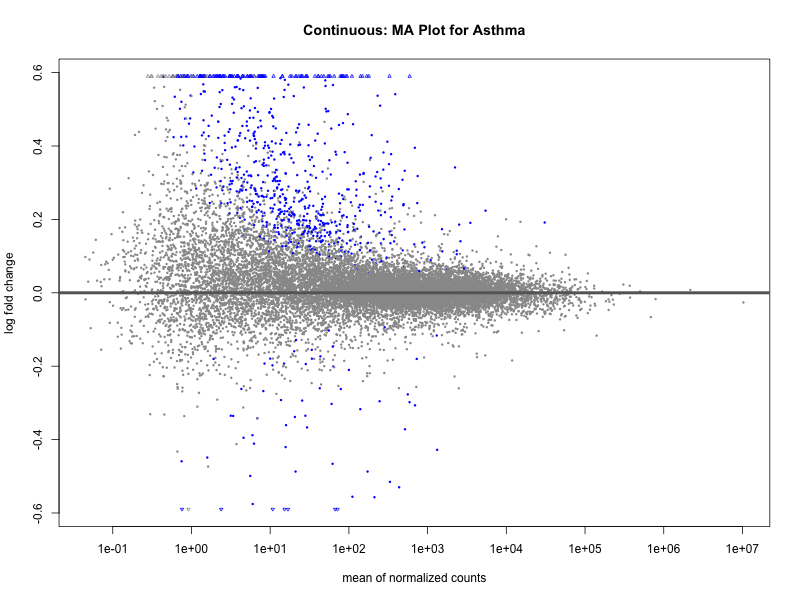
# plot the MA-plot for the current trait
png(paste0("ma_plot_asthma.png"), width = 800, height = 600)
plotMA(res, main = paste("Continuous: MA Plot for Asthma"))
dev.off()
  
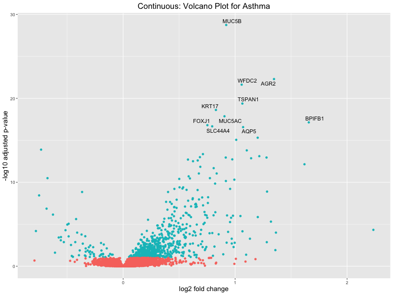
# volcano plot
res_tableOE <- as.data.frame(res)
res_tableOE$gene_name <- raw_count_df$Description[keep_genes]
res_tableOE <- mutate(res_tableOE, threshold_OE = padj < 0.1)
res_tableOE <- res_tableOE %>% arrange(padj) %>% mutate(genelabels = "")
res_tableOE$genelabels[1:10] <- res_tableOE$gene_name[1:10]
  
volcano_plot <- ggplot(res_tableOE, aes(x = log2FoldChange, y = -log10(padj))) +
    geom_point(aes(colour = threshold_OE)) +
    geom_text_repel(aes(label = genelabels)) +
    ggtitle(paste("Continuous: Volcano Plot for Asthma")) +
    xlab("log2 fold change") + 
    ylab("-log10 adjusted p-value") +
    theme(legend.position = "none",
          plot.title = element_text(size = rel(1.5), hjust = 0.5),
          axis.title = element_text(size = rel(1.25)))
  
# Save the volcano plot
png(paste0("volcano_plot_asthma.png"), width = 800, height = 600)
print(volcano_plot)
dev.off()

GO enrichment Analysis

file <- "analysis/asthma_wb/differential_expression_asthma_results.csv"

res_tableOE <- read.csv(file, header = T, row.names = 1)
  
deGenes <- res_tableOE[res_tableOE$padj < 0.1 & 
                         abs(res_tableOE$log2FoldChange) >= 0.5, ]
deGenes$gene_id <- gsub("\\.\\d+$", "", rownames(deGenes))

# Separate upregulated and downregulated genes
upregulated_genes <- deGenes[deGenes$log2FoldChange > 0, ]$gene_id
downregulated_genes <- deGenes[deGenes$log2FoldChange < 0, ]$gene_id
  
# Run GO enrichment for upregulated genes
gse_up <- enrichGO(gene = upregulated_genes, ont = "BP", 
                   OrgDb = "org.Hs.eg.db", keyType = "ENSEMBL", readable = T)

# Run GO enrichment for downregulated genes
gse_down <- enrichGO(gene = downregulated_genes, ont = "BP", 
                     OrgDb = "org.Hs.eg.db", keyType = "ENSEMBL", readable = T)
  
# Convert enrichment results to data frames and calculate additional ratios
gse_up <- as.data.frame(gse_up)
gse_down <- as.data.frame(gse_down)

gse_up$GeneRatio_num <- as.numeric(sapply(strsplit(gse_up$GeneRatio, "/"), function(x) x[1])) / 
                        as.numeric(sapply(strsplit(gse_up$GeneRatio, "/"), function(x) x[2]))
gse_up$BgRatio_num <- as.numeric(sapply(strsplit(gse_up$BgRatio, "/"), function(x) x[1])) / 
                        as.numeric(sapply(strsplit(gse_up$BgRatio, "/"), function(x) x[2]))
gse_up <- cbind(gse_up, FoldEnrich = gse_up$GeneRatio_num / gse_up$BgRatio_num)

gse_down$GeneRatio_num <- as.numeric(sapply(strsplit(gse_down$GeneRatio, "/"), function(x) x[1])) / 
                          as.numeric(sapply(strsplit(gse_down$GeneRatio, "/"), function(x) x[2]))
gse_down$BgRatio_num <- as.numeric(sapply(strsplit(gse_down$BgRatio, "/"), function(x) x[1])) / 
                          as.numeric(sapply(strsplit(gse_down$BgRatio, "/"), function(x) x[2]))
gse_down <- cbind(gse_down, FoldEnrich = gse_down$GeneRatio_num / gse_down$BgRatio_num)

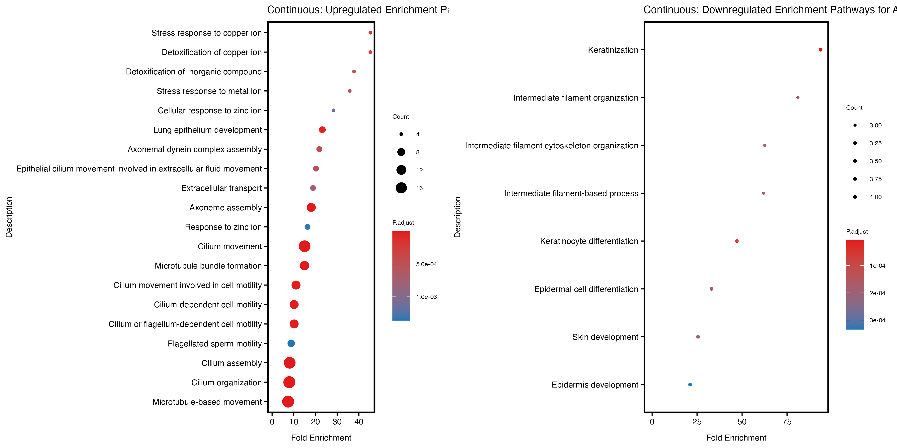
if (nrow(gse_up) >= 20) {
    enrich_plot_up <- plotEnrich(gse_up[1:20,], plot_type = "dot", scale_ratio = 0.5) +
    labs(title = "Continuous: Upregulated Enrichment Pathways for Asthma") + 
    theme(plot.title = element_text(size = 10)) 
}else{
    enrich_plot_up <- plotEnrich(gse_up, plot_type = "dot", scale_ratio = 0.5) +
    labs(title = "Continuous: Upregulated Enrichment Pathways for Asthma") + 
    theme(plot.title = element_text(size = 10)) 
}

if (nrow(gse_down) >= 20) {
    enrich_plot_down <- plotEnrich(gse_down[1:20,], plot_type = "dot", scale_ratio = 0.5) +
    labs(title = "Continuous: Downregulated Enrichment Pathways for Asthma") + 
    theme(plot.title = element_text(size = 10)) 
}else{
    enrich_plot_down <- plotEnrich(gse_down, plot_type = "dot", scale_ratio = 0.5) +
    labs(title = "Continuous: Downregulated Enrichment Pathways for Asthma") + 
    theme(plot.title = element_text(size = 10)) 
}

# Arrange the two plots side by side
combined_plot <- grid.arrange(enrich_plot_up, enrich_plot_down, ncol = 2)

# Save the combined plot
ggsave("enrichment_plot_asthma.png", plot = combined_plot, width = 12, height = 6)

# Save the GO enrichment results to CSV
write.csv(gse_up, "GO_enrichment_asthma_upregulated.csv")
write.csv(gse_down, "GO_enrichment_asthma_downregulated.csv")

Quantile PRS

DESeq2 Differential Expression

metadata_file <- "analysis/metadata_asthma_quantile.txt"
metadata <- read.csv(metadata_file, header = T, sep = "\t", stringsAsFactors = T)
metadata$sex <- as.factor(metadata$sex)

# Create the DESeqDataSet for the current trait
dds <- DESeqDataSetFromMatrix(
  countData = as.matrix(final_count),
  colData = metadata,
  design = as.formula("~ PC1 + PC2 + PC3 + PC4 + PC5 + sex + asthma")
  )
rownames(dds) <- id
  
# Run DESeq2 analysis
dds <- DESeq(dds, parallel = TRUE, BPPARAM = MulticoreParam(4))
  
# Get the results for the current trait
res <- results(dds)
  
# Save the results to a file
write.csv(res, "differential_expression_asthma_quantile_results.csv")
  
# print a summary of the results
print(paste("Results for trait: asthma"))
print(summary(res))
  
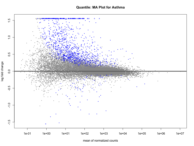
# plot the MA-plot for the current trait
png(paste0("ma_plot_quantile_asthma.png"), width = 800, height = 600)
plotMA(res, main = paste("Quantile: MA Plot for Asthma"))
dev.off()
  
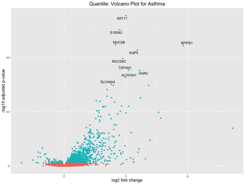
# volcano plot
res_tableOE <- as.data.frame(res)
res_tableOE$gene_name <- raw_count_df$Description[keep_genes]
res_tableOE <- mutate(res_tableOE, threshold_OE = padj < 0.1)
res_tableOE <- res_tableOE %>% arrange(padj) %>% mutate(genelabels = "")
res_tableOE$genelabels[1:10] <- res_tableOE$gene_name[1:10]
  
volcano_plot <- ggplot(res_tableOE, aes(x = log2FoldChange, y = -log10(padj))) +
    geom_point(aes(colour = threshold_OE)) +
    geom_text_repel(aes(label = genelabels)) +
    ggtitle(paste("Quantile: Volcano Plot for Asthma")) +
    xlab("log2 fold change") + 
    ylab("-log10 adjusted p-value") +
    theme(legend.position = "none",
          plot.title = element_text(size = rel(1.5), hjust = 0.5),
          axis.title = element_text(size = rel(1.25)))
  
# Save the volcano plot
png(paste0("volcano_plot_quantile_asthma.png"), width = 800, height = 600)
print(volcano_plot)
dev.off()

GO enrichment Analysis

file <- "analysis/asthma_wb/differential_expression_asthma_quantile_results.csv"

res_tableOE <- read.csv(file, header = T, row.names = 1)
  
deGenes <- res_tableOE[res_tableOE$padj < 0.1 & 
                         abs(res_tableOE$log2FoldChange) >= 0.5, ]
deGenes$gene_id <- gsub("\\.\\d+$", "", rownames(deGenes))

# Separate upregulated and downregulated genes
upregulated_genes <- deGenes[deGenes$log2FoldChange > 0, ]$gene_id
downregulated_genes <- deGenes[deGenes$log2FoldChange < 0, ]$gene_id
  
# Run GO enrichment for upregulated genes
gse_up <- enrichGO(gene = upregulated_genes, ont = "BP", 
                   OrgDb = "org.Hs.eg.db", keyType = "ENSEMBL", readable = T)

# Run GO enrichment for downregulated genes
gse_down <- enrichGO(gene = downregulated_genes, ont = "BP", 
                     OrgDb = "org.Hs.eg.db", keyType = "ENSEMBL", readable = T)
  
# Convert enrichment results to data frames and calculate additional ratios
gse_up <- as.data.frame(gse_up)
gse_down <- as.data.frame(gse_down)

gse_up$GeneRatio_num <- as.numeric(sapply(strsplit(gse_up$GeneRatio, "/"), function(x) x[1])) / 
                        as.numeric(sapply(strsplit(gse_up$GeneRatio, "/"), function(x) x[2]))
gse_up$BgRatio_num <- as.numeric(sapply(strsplit(gse_up$BgRatio, "/"), function(x) x[1])) / 
                        as.numeric(sapply(strsplit(gse_up$BgRatio, "/"), function(x) x[2]))
gse_up <- cbind(gse_up, FoldEnrich = gse_up$GeneRatio_num / gse_up$BgRatio_num)

gse_down$GeneRatio_num <- as.numeric(sapply(strsplit(gse_down$GeneRatio, "/"), function(x) x[1])) / 
                          as.numeric(sapply(strsplit(gse_down$GeneRatio, "/"), function(x) x[2]))
gse_down$BgRatio_num <- as.numeric(sapply(strsplit(gse_down$BgRatio, "/"), function(x) x[1])) / 
                          as.numeric(sapply(strsplit(gse_down$BgRatio, "/"), function(x) x[2]))
gse_down <- cbind(gse_down, FoldEnrich = gse_down$GeneRatio_num / gse_down$BgRatio_num)

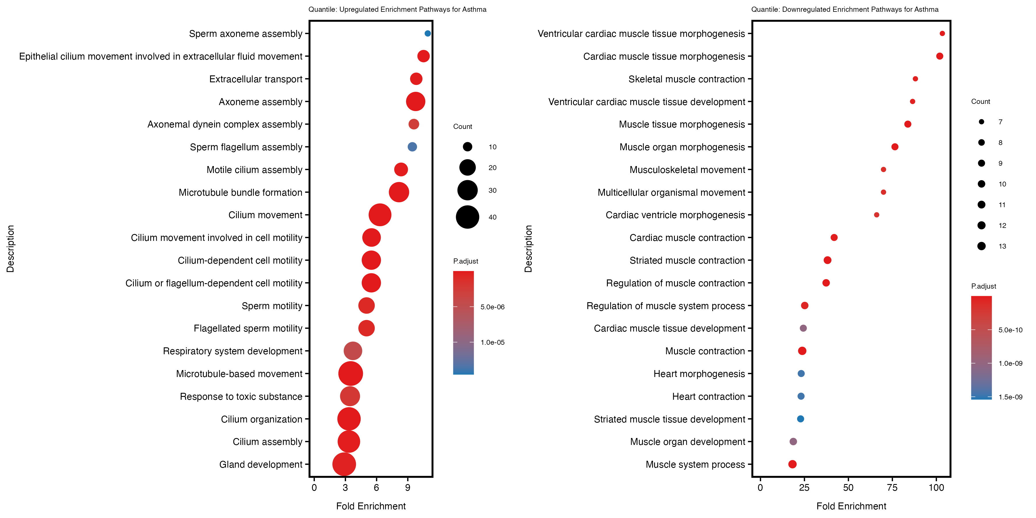
if (nrow(gse_up) >= 20) {
    enrich_plot_up <- plotEnrich(gse_up[1:20,], plot_type = "dot", scale_ratio = 0.4) +
    labs(title = "Quantile: Upregulated Enrichment Pathways for Asthma") + 
    theme(plot.title = element_text(size = 6)) 
}else{
    enrich_plot_up <- plotEnrich(gse_up, plot_type = "dot", scale_ratio = 0.4) +
    labs(title = "Quantile: Upregulated Enrichment Pathways for Asthma") + 
    theme(plot.title = element_text(size = 6)) 
}

if (nrow(gse_down) >= 20) {
    enrich_plot_down <- plotEnrich(gse_down[1:20,], plot_type = "dot", scale_ratio = 0.4) +
    labs(title = "Quantile: Downregulated Enrichment Pathways for Asthma") + 
    theme(plot.title = element_text(size = 6)) 
}else{
    enrich_plot_down <- plotEnrich(gse_down, plot_type = "dot", scale_ratio = 0.4) +
    labs(title = "Quantile: Downregulated Enrichment Pathways for Asthma") + 
    theme(plot.title = element_text(size = 6)) 
}

# Arrange the two plots side by side
combined_plot <- grid.arrange(enrich_plot_up, enrich_plot_down, ncol = 2)

# Save the combined plot
ggsave("enrichment_plot_quantile_asthma.png", plot = combined_plot, width = 12, height = 6)

# Save the GO enrichment results to CSV
write.csv(gse_up, "GO_enrichment_quantile_asthma_upregulated.csv")
write.csv(gse_down, "GO_enrichment_quantile_asthma_downregulated.csv")

Model 2: expression ~ PRS + sex + expression PCs + 2 genotype PCs

Obtain genotype PCs

# Load the gene expression data
gene_expr_file <- "data/gene_reads_2017-06-05_v8_whole_blood.gct"
raw_count_df <- fread(gene_expr_file, header = TRUE, sep = "\t", drop = "id")

# load protein_coding list
protein_coding <- fread("data/protein-coding_gene.txt", 
                        sep = "\t")
protein_coding <- protein_coding[, c("symbol", "ensembl_gene_id")]

# keep only protein-coding genes
raw_count_df <- raw_count_df[raw_count_df$Description %in% protein_coding$symbol, ]

id <- raw_count_df$Name
raw_count <- raw_count_df[, -c(1:2)]

# modify GTEx sample names matching names used in PRS data
colnames(raw_count) <- sub("^(GTEX-[^-.]+).*", "\\1", colnames(raw_count))

matching_samples <- intersect(rownames(metadata), colnames(raw_count))
final_count <- raw_count[ , ..matching_samples]

# prefilter: keep only rows that have a count of at least 10
keep_genes <- rowSums(final_count >= 10) > 0
final_count <- final_count[keep_genes, ]
id <- id[keep_genes]
dim(final_count)

[1] 16893   670

# obtain genotype PCs
geno_pc <- read.table("data/pca.eigenvec")
names(geno_pc) = c("FID","IID",paste0("geno_PC", c(1:(ncol(geno_pc)-2))))
geno_pc <- geno_pc[geno_pc$FID %in% matching_samples, ]

eigenval <- scan("data/pca.eigenval")
pve <- data.frame(PC = 1:20, pve = eigenval/sum(eigenval)*100)

ggplot(geno_pc) + geom_point(aes(x = geno_PC1, y = geno_PC2)) + 
  labs(x = paste0("PC1 (", signif(pve$pve[1], 3), "%)"), 
       y = paste0("PC2 (", signif(pve$pve[2], 3), "%)")) + theme_classic()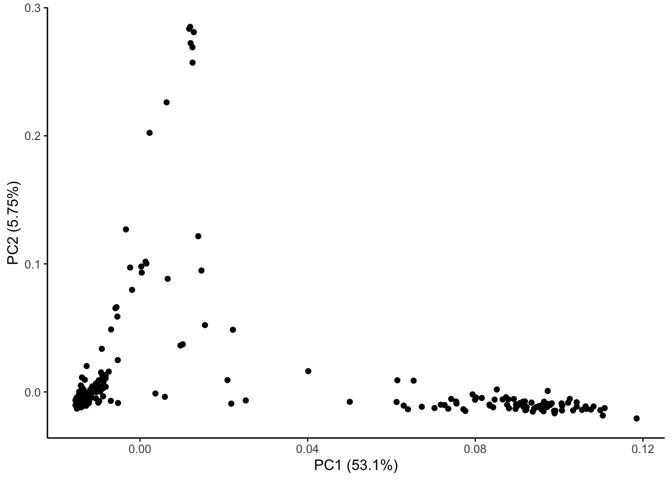

Version	Author	Date
36ca2c8	ElisaChen	2025-05-30

ggplot(geno_pc) + geom_point(aes(x = geno_PC1, y = geno_PC3)) + 
    labs(x = paste0("PC1 (", signif(pve$pve[1], 3), "%)"), 
         y = paste0("PC3 (", signif(pve$pve[3], 3), "%)")) + theme_classic()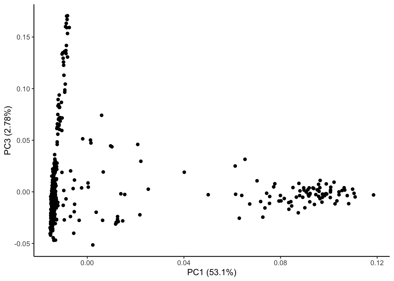

Version	Author	Date
36ca2c8	ElisaChen	2025-05-30

ggplot(pve, aes(PC, pve)) + geom_point() + geom_line() +
  labs(x = "Genotype PC", y = "Percentage variance explained") + theme_classic()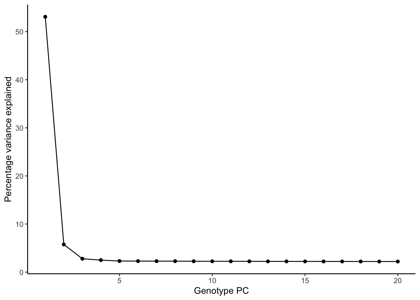

Version	Author	Date
36ca2c8	ElisaChen	2025-05-30

Continuous PRS

DESeq2 Differential Expression

metadata_file <- "analysis/metadata_asthma.txt"
metadata <- read.csv(metadata_file, header = T, sep = "\t", stringsAsFactors = T)
metadata$sex <- as.factor(metadata$sex)

metadata <- cbind(metadata, geno_pc[,3:ncol(geno_pc)])

# Standardize PRS for the current trait
prs_trait <- scale(metadata$asthma)

# Add the standardized PRS to the metadata for continuous trait
metadata$asthma <- prs_trait

# Create the DESeqDataSet for the current trait
dds <- DESeqDataSetFromMatrix(
  countData = as.matrix(final_count),  # Raw counts
  colData = metadata[, 1:9],
  design = as.formula("~ PC1 + PC2 + PC3 + PC4 + PC5 + sex + geno_PC1 + geno_PC2 + asthma")
)
rownames(dds) <- id

# Run DESeq2 analysis
dds <- DESeq(dds, parallel = TRUE, BPPARAM = MulticoreParam(4))

# Get the results for the current trait
res <- results(dds)
  
# Save the results to a file
write.csv(res, "differential_expression_asthma_results_M2.csv")
  
# print a summary of the results
print("Results for trait: Asthma")
print(summary(res))
  
# plot the MA-plot for the current trait
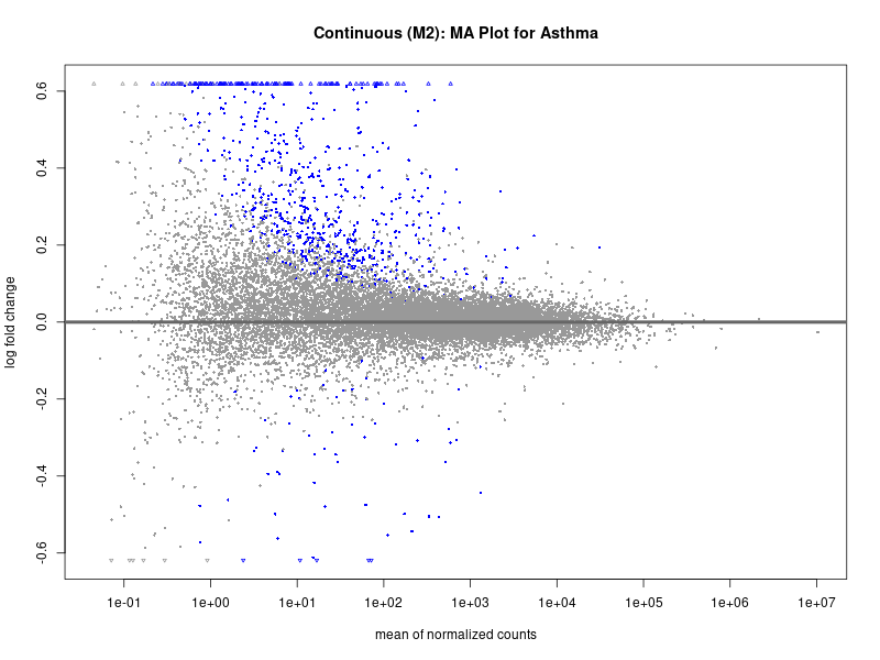
png(paste0("ma_plot_asthma_M2.png"), width = 800, height = 600)
plotMA(res, main = "Continuous (M2): MA Plot for Asthma")
dev.off()
  
# volcano plot
res_tableOE <- as.data.frame(res)
res_tableOE$gene_name <- raw_count_df$Description[keep_genes]
res_tableOE <- mutate(res_tableOE, threshold_OE = padj < 0.1)
res_tableOE <- res_tableOE %>% arrange(padj) %>% mutate(genelabels = "")
res_tableOE$genelabels[1:10] <- res_tableOE$gene_name[1:10]
  
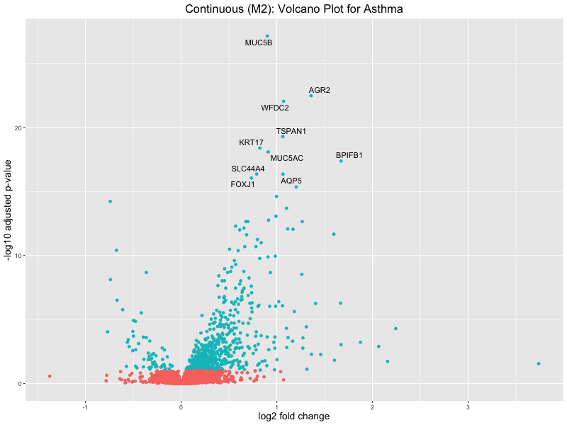
volcano_plot <- ggplot(res_tableOE, aes(x = log2FoldChange, y = -log10(padj))) +
  geom_point(aes(colour = threshold_OE)) +
  geom_text_repel(aes(label = genelabels)) +
  ggtitle("Continuous (M2): Volcano Plot for Asthma") +
    xlab("log2 fold change") + 
    ylab("-log10 adjusted p-value") +
    theme(legend.position = "none",
          plot.title = element_text(size = rel(1.5), hjust = 0.5),
          axis.title = element_text(size = rel(1.25)))
  
# Save the volcano plot
png(paste0("volcano_plot_asthma_M2.png"), width = 800, height = 600)
print(volcano_plot)
dev.off()

GO enrichment Analysis

file <- "analysis/asthma_wb/differential_expression_asthma_results_M2.csv"

res_tableOE <- read.csv(file, header = T, row.names = 1)
  
deGenes <- res_tableOE[res_tableOE$padj < 0.1 & 
                         abs(res_tableOE$log2FoldChange) >= 0.5, ]
deGenes$gene_id <- gsub("\\.\\d+$", "", rownames(deGenes))

# Separate upregulated and downregulated genes
upregulated_genes <- deGenes[deGenes$log2FoldChange > 0, ]$gene_id
downregulated_genes <- deGenes[deGenes$log2FoldChange < 0, ]$gene_id
  
# Run GO enrichment for upregulated genes
gse_up <- enrichGO(gene = upregulated_genes, ont = "BP", 
                   OrgDb = "org.Hs.eg.db", keyType = "ENSEMBL", readable = T)

# Run GO enrichment for downregulated genes
gse_down <- enrichGO(gene = downregulated_genes, ont = "BP", 
                     OrgDb = "org.Hs.eg.db", keyType = "ENSEMBL", readable = T)
  
# Convert enrichment results to data frames and calculate additional ratios
gse_up <- as.data.frame(gse_up)
gse_down <- as.data.frame(gse_down)

gse_up$GeneRatio_num <- as.numeric(sapply(strsplit(gse_up$GeneRatio, "/"), function(x) x[1])) / 
                        as.numeric(sapply(strsplit(gse_up$GeneRatio, "/"), function(x) x[2]))
gse_up$BgRatio_num <- as.numeric(sapply(strsplit(gse_up$BgRatio, "/"), function(x) x[1])) / 
                        as.numeric(sapply(strsplit(gse_up$BgRatio, "/"), function(x) x[2]))
gse_up <- cbind(gse_up, FoldEnrich = gse_up$GeneRatio_num / gse_up$BgRatio_num)

gse_down$GeneRatio_num <- as.numeric(sapply(strsplit(gse_down$GeneRatio, "/"), function(x) x[1])) / 
                          as.numeric(sapply(strsplit(gse_down$GeneRatio, "/"), function(x) x[2]))
gse_down$BgRatio_num <- as.numeric(sapply(strsplit(gse_down$BgRatio, "/"), function(x) x[1])) / 
                          as.numeric(sapply(strsplit(gse_down$BgRatio, "/"), function(x) x[2]))
gse_down <- cbind(gse_down, FoldEnrich = gse_down$GeneRatio_num / gse_down$BgRatio_num)

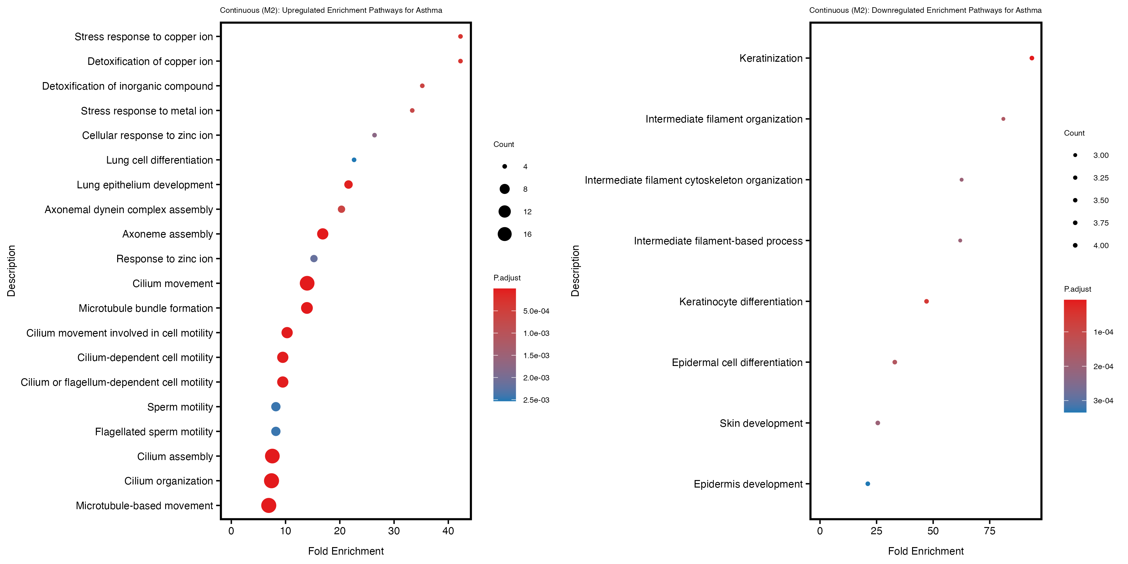
if (nrow(gse_up) >= 20) {
    enrich_plot_up <- plotEnrich(gse_up[1:20,], plot_type = "dot", scale_ratio = 0.5) +
    labs(title = "Continuous (M2): Upregulated Enrichment Pathways for Asthma") + 
    theme(plot.title = element_text(size = 6)) 
}else{
    enrich_plot_up <- plotEnrich(gse_up, plot_type = "dot", scale_ratio = 0.5) +
    labs(title = "Continuous (M2): Upregulated Enrichment Pathways for Asthma") + 
    theme(plot.title = element_text(size = 6)) 
}

if (nrow(gse_down) >= 20) {
    enrich_plot_down <- plotEnrich(gse_down[1:20,], plot_type = "dot", scale_ratio = 0.5) +
    labs(title = "Continuous (M2): Downregulated Enrichment Pathways for Asthma") + 
    theme(plot.title = element_text(size = 6)) 
}else{
    enrich_plot_down <- plotEnrich(gse_down, plot_type = "dot", scale_ratio = 0.5) +
    labs(title = "Continuous (M2): Downregulated Enrichment Pathways for Asthma") + 
    theme(plot.title = element_text(size = 6)) 
}

# Arrange the two plots side by side
combined_plot <- grid.arrange(enrich_plot_up, enrich_plot_down, ncol = 2)

# Save the combined plot
ggsave("enrichment_plot_asthma_M2.png", plot = combined_plot, width = 12, height = 6)

# Save the GO enrichment results to CSV
write.csv(gse_up, "GO_enrichment_asthma_upregulated_M2.csv")
write.csv(gse_down, "GO_enrichment_asthma_downregulated_M2.csv")

Quantile PRS

DESeq2 Differential Expression

metadata_file <- "analysis/metadata_asthma_quantile.txt"
metadata <- read.csv(metadata_file, header = T, sep = "\t", stringsAsFactors = T)
metadata$sex <- as.factor(metadata$sex)

metadata <- cbind(metadata, geno_pc[,3:ncol(geno_pc)])

# Create the DESeqDataSet for the current trait
dds <- DESeqDataSetFromMatrix(
  countData = as.matrix(final_count),  # Raw counts
  colData = metadata[, 1:9],
  design = as.formula("~ PC1 + PC2 + PC3 + PC4 + PC5 + sex + geno_PC1 + geno_PC2 + asthma")
)
rownames(dds) <- id

# Run DESeq2 analysis
dds <- DESeq(dds, parallel = TRUE, BPPARAM = MulticoreParam(4))

# Get the results for the current trait
res <- results(dds)
  
# Save the results to a file
write.csv(res, "differential_expression_asthma_quantile_results_M2.csv")
  
# print a summary of the results
print("Results for trait: Asthma")
print(summary(res))
  
# plot the MA-plot for the current trait
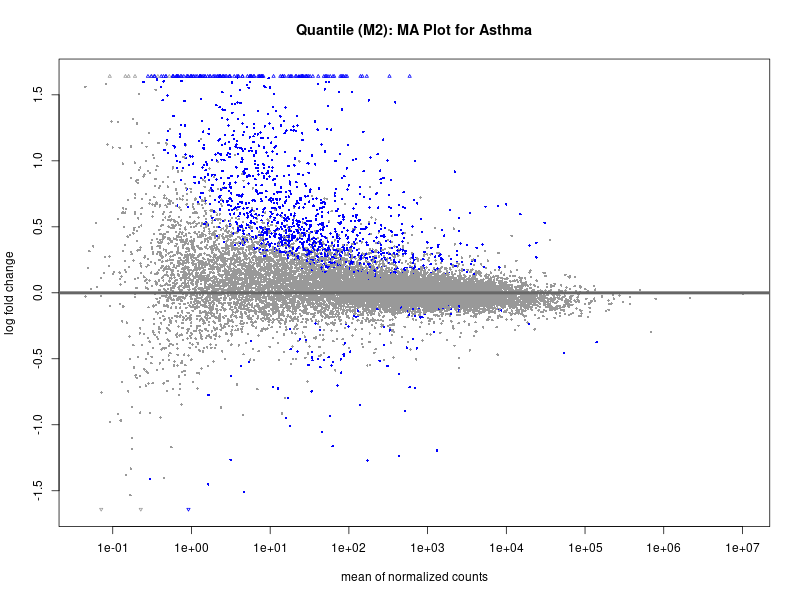
png(paste0("ma_plot_quantile_asthma_M2.png"), width = 800, height = 600)
plotMA(res, main = "Quantile (M2): MA Plot for Asthma")
dev.off()
  
# volcano plot
res_tableOE <- as.data.frame(res)
res_tableOE$gene_name <- raw_count_df$Description[keep_genes]
res_tableOE <- mutate(res_tableOE, threshold_OE = padj < 0.1)
res_tableOE <- res_tableOE %>% arrange(padj) %>% mutate(genelabels = "")
res_tableOE$genelabels[1:10] <- res_tableOE$gene_name[1:10]
  
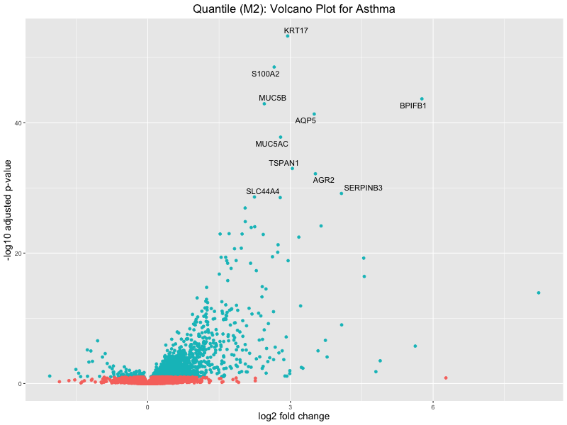
volcano_plot <- ggplot(res_tableOE, aes(x = log2FoldChange, y = -log10(padj))) +
  geom_point(aes(colour = threshold_OE)) +
  geom_text_repel(aes(label = genelabels)) +
  ggtitle("Quantile (M2): Volcano Plot for Asthma") +
    xlab("log2 fold change") + 
    ylab("-log10 adjusted p-value") +
    theme(legend.position = "none",
          plot.title = element_text(size = rel(1.5), hjust = 0.5),
          axis.title = element_text(size = rel(1.25)))
  
# Save the volcano plot
png(paste0("volcano_plot_quantile_asthma_M2.png"), width = 800, height = 600)
print(volcano_plot)
dev.off()

GO enrichment Analysis

file <- "analysis/asthma_wb/differential_expression_asthma_quantile_results_M2.csv"

res_tableOE <- read.csv(file, header = T, row.names = 1)
  
deGenes <- res_tableOE[res_tableOE$padj < 0.1 & 
                         abs(res_tableOE$log2FoldChange) >= 0.5, ]
deGenes$gene_id <- gsub("\\.\\d+$", "", rownames(deGenes))

# Separate upregulated and downregulated genes
upregulated_genes <- deGenes[deGenes$log2FoldChange > 0, ]$gene_id
downregulated_genes <- deGenes[deGenes$log2FoldChange < 0, ]$gene_id
  
# Run GO enrichment for upregulated genes
gse_up <- enrichGO(gene = upregulated_genes, ont = "BP", 
                   OrgDb = "org.Hs.eg.db", keyType = "ENSEMBL", readable = T)

# Run GO enrichment for downregulated genes
gse_down <- enrichGO(gene = downregulated_genes, ont = "BP", 
                     OrgDb = "org.Hs.eg.db", keyType = "ENSEMBL", readable = T)
  
# Convert enrichment results to data frames and calculate additional ratios
gse_up <- as.data.frame(gse_up)
gse_down <- as.data.frame(gse_down)

gse_up$GeneRatio_num <- as.numeric(sapply(strsplit(gse_up$GeneRatio, "/"), function(x) x[1])) / 
                        as.numeric(sapply(strsplit(gse_up$GeneRatio, "/"), function(x) x[2]))
gse_up$BgRatio_num <- as.numeric(sapply(strsplit(gse_up$BgRatio, "/"), function(x) x[1])) / 
                        as.numeric(sapply(strsplit(gse_up$BgRatio, "/"), function(x) x[2]))
gse_up <- cbind(gse_up, FoldEnrich = gse_up$GeneRatio_num / gse_up$BgRatio_num)

gse_down$GeneRatio_num <- as.numeric(sapply(strsplit(gse_down$GeneRatio, "/"), function(x) x[1])) / 
                          as.numeric(sapply(strsplit(gse_down$GeneRatio, "/"), function(x) x[2]))
gse_down$BgRatio_num <- as.numeric(sapply(strsplit(gse_down$BgRatio, "/"), function(x) x[1])) / 
                          as.numeric(sapply(strsplit(gse_down$BgRatio, "/"), function(x) x[2]))
gse_down <- cbind(gse_down, FoldEnrich = gse_down$GeneRatio_num / gse_down$BgRatio_num)

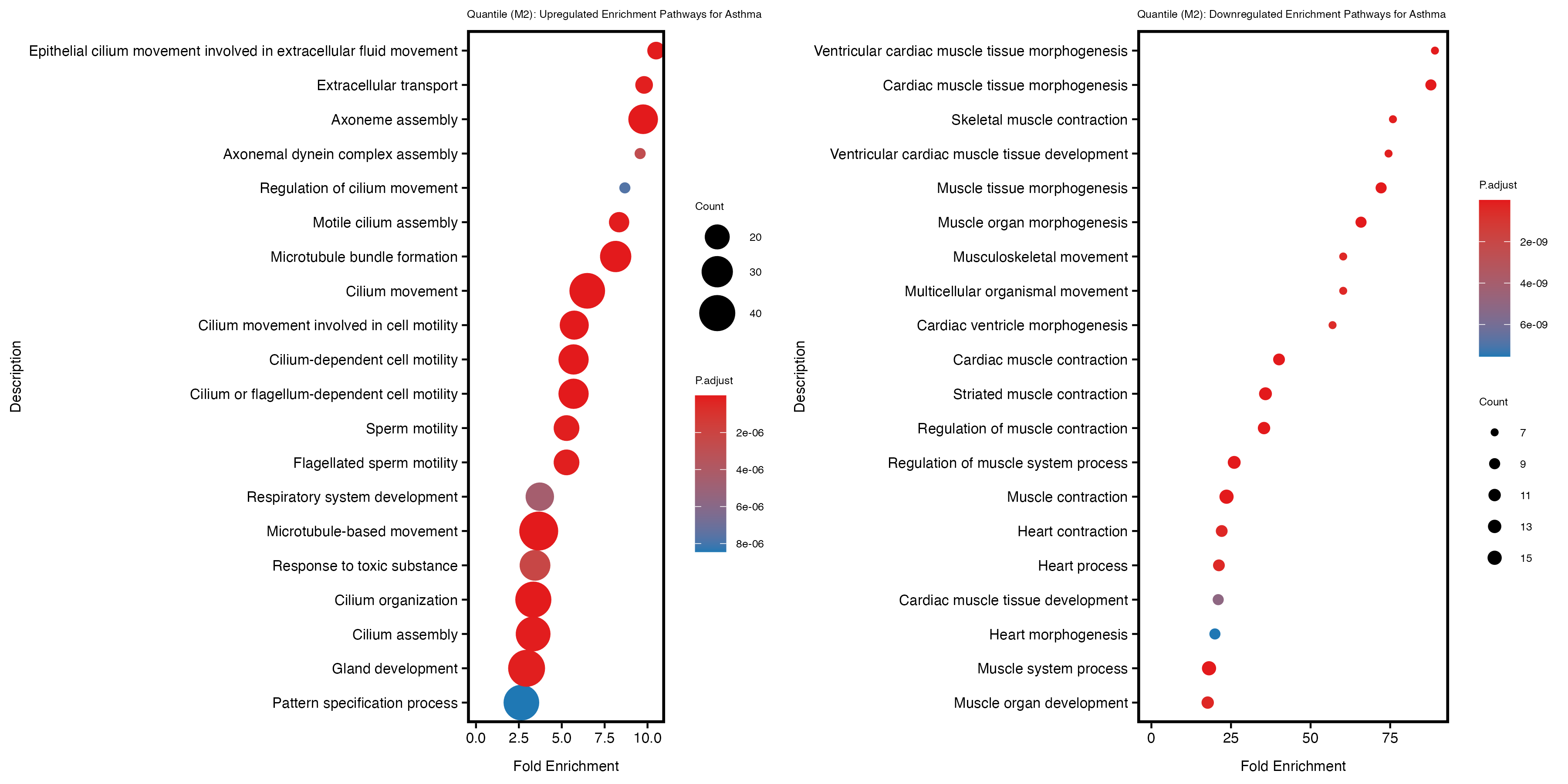
if (nrow(gse_up) >= 20) {
    enrich_plot_up <- plotEnrich(gse_up[1:20,], plot_type = "dot", scale_ratio = 0.4) +
    labs(title = "Quantile (M2): Upregulated Enrichment Pathways for Asthma") + 
    theme(plot.title = element_text(size = 6)) 
}else{
    enrich_plot_up <- plotEnrich(gse_up, plot_type = "dot", scale_ratio = 0.4) +
    labs(title = "Quantile (M2): Upregulated Enrichment Pathways for Asthma") + 
    theme(plot.title = element_text(size = 6)) 
}

if (nrow(gse_down) >= 20) {
    enrich_plot_down <- plotEnrich(gse_down[1:20,], plot_type = "dot", scale_ratio = 0.4) +
    labs(title = "Quantile (M2): Downregulated Enrichment Pathways for Asthma") + 
    theme(plot.title = element_text(size = 6)) 
}else{
    enrich_plot_down <- plotEnrich(gse_down, plot_type = "dot", scale_ratio = 0.4) +
    labs(title = "Quantile (M2): Downregulated Enrichment Pathways for Asthma") + 
    theme(plot.title = element_text(size = 6)) 
}

# Arrange the two plots side by side
combined_plot <- grid.arrange(enrich_plot_up, enrich_plot_down, ncol = 2)

# Save the combined plot
ggsave("enrichment_plot_quantile_asthma_M2.png", plot = combined_plot, width = 12, height = 6)

# Save the GO enrichment results to CSV
write.csv(gse_up, "GO_enrichment_quantile_asthma_upregulated_M2.csv")
write.csv(gse_down, "GO_enrichment_quantil_asthma_downregulated_M2.csv")

Results

Summary table

Summary of Differential Expression and Enriched Pathways for Asthma PRS Models
Model	Significant DE genes	Up-regulated genes	Down-regulated genes	Up-regulated GO pathways	Down-regulated GO pathways
continuous	575	525	50	43	8
continuous_M2	587	536	51	44	8
quantile	1028	987	41	251	64
quantile_M2	1037	993	44	275	61

Model 1: Adjust without genotype PCs

Continuous PRS

Quantile PRS

Model 2: Adjust with genotype PCs

Continuous PRS

Quantile PRS

sessionInfo()

R version 4.2.2 (2022-10-31)
Platform: x86_64-apple-darwin17.0 (64-bit)
Running under: macOS Big Sur ... 10.16

Matrix products: default
BLAS:   /Library/Frameworks/R.framework/Versions/4.2/Resources/lib/libRblas.0.dylib
LAPACK: /Library/Frameworks/R.framework/Versions/4.2/Resources/lib/libRlapack.dylib

locale:
[1] en_US.UTF-8/en_US.UTF-8/en_US.UTF-8/C/en_US.UTF-8/en_US.UTF-8

attached base packages:
[1] stats4    stats     graphics  grDevices utils     datasets  methods  
[8] base     

other attached packages:
 [1] gridExtra_2.3               clusterProfiler_4.6.2      
 [3] enrichplot_1.18.4           org.Hs.eg.db_3.16.0        
 [5] AnnotationDbi_1.60.2        genekitr_1.2.8             
 [7] ggrepel_0.9.6               BiocParallel_1.32.6        
 [9] DESeq2_1.38.3               SummarizedExperiment_1.28.0
[11] Biobase_2.58.0              MatrixGenerics_1.10.0      
[13] matrixStats_1.2.0           GenomicRanges_1.50.2       
[15] GenomeInfoDb_1.34.9         IRanges_2.32.0             
[17] S4Vectors_0.36.2            BiocGenerics_0.44.0        
[19] corrplot_0.95               lubridate_1.9.4            
[21] forcats_1.0.0               stringr_1.5.1              
[23] dplyr_1.1.4                 purrr_1.0.2                
[25] readr_2.1.5                 tidyr_1.3.1                
[27] tibble_3.2.1                ggplot2_3.5.1              
[29] tidyverse_2.0.0             data.table_1.16.4          
[31] workflowr_1.7.1            

loaded via a namespace (and not attached):
  [1] shadowtext_0.1.4       fastmatch_1.1-6        plyr_1.8.9            
  [4] igraph_1.5.1           lazyeval_0.2.2         splines_4.2.2         
  [7] usethis_3.1.0          urltools_1.7.3         digest_0.6.37         
 [10] yulab.utils_0.2.0      htmltools_0.5.8.1      GOSemSim_2.24.0       
 [13] viridis_0.6.5          GO.db_3.16.0           magrittr_2.0.3        
 [16] memoise_2.0.1          remotes_2.5.0          openxlsx_4.2.5.2      
 [19] tzdb_0.4.0             Biostrings_2.66.0      annotate_1.76.0       
 [22] graphlayouts_1.0.1     vroom_1.6.5            timechange_0.3.0      
 [25] prettyunits_1.2.0      colorspace_2.1-1       blob_1.2.4            
 [28] xfun_0.50              callr_3.7.6            crayon_1.5.3          
 [31] RCurl_1.98-1.16        jsonlite_1.8.9         scatterpie_0.2.4      
 [34] ape_5.7-1              glue_1.8.0             polyclip_1.10-7       
 [37] gtable_0.3.6           zlibbioc_1.44.0        XVector_0.38.0        
 [40] DelayedArray_0.24.0    pkgbuild_1.4.6         scales_1.3.0          
 [43] DOSE_3.24.2            DBI_1.2.3              miniUI_0.1.1.1        
 [46] Rcpp_1.0.14            progress_1.2.3         viridisLite_0.4.2     
 [49] xtable_1.8-4           gridGraphics_0.5-1     tidytree_0.4.6        
 [52] europepmc_0.4.3        bit_4.5.0.1            profvis_0.4.0         
 [55] htmlwidgets_1.6.4      httr_1.4.7             fgsea_1.24.0          
 [58] RColorBrewer_1.1-3     ellipsis_0.3.2         urlchecker_1.0.1      
 [61] pkgconfig_2.0.3        XML_3.99-0.18          farver_2.1.2          
 [64] sass_0.4.9             locfit_1.5-9.8         labeling_0.4.3        
 [67] ggplotify_0.1.2        tidyselect_1.2.1       rlang_1.1.5           
 [70] reshape2_1.4.4         later_1.4.1            munsell_0.5.1         
 [73] tools_4.2.2            cachem_1.1.0           downloader_0.4        
 [76] cli_3.6.3              generics_0.1.3         RSQLite_2.3.9         
 [79] gson_0.1.0             devtools_2.4.5         evaluate_1.0.3        
 [82] fastmap_1.2.0          yaml_2.3.10            ggtree_3.6.2          
 [85] processx_3.8.5         knitr_1.49             bit64_4.6.0-1         
 [88] fs_1.6.5               tidygraph_1.3.0        zip_2.3.2             
 [91] KEGGREST_1.38.0        ggraph_2.1.0           nlme_3.1-160          
 [94] mime_0.12              whisker_0.4.1          aplot_0.2.4           
 [97] ggvenn_0.1.10          xml2_1.3.6             compiler_4.2.2        
[100] rstudioapi_0.17.1      png_0.1-8              treeio_1.22.0         
[103] tweenr_2.0.3           geneplotter_1.76.0     bslib_0.9.0           
[106] stringi_1.8.4          ps_1.8.1               lattice_0.22-6        
[109] Matrix_1.6-4           vctrs_0.6.5            pillar_1.10.1         
[112] lifecycle_1.0.4        triebeard_0.4.1        jquerylib_0.1.4       
[115] cowplot_1.1.3          bitops_1.0-9           httpuv_1.6.15         
[118] patchwork_1.3.0        qvalue_2.30.0          R6_2.5.1              
[121] promises_1.3.2         sessioninfo_1.2.2      codetools_0.2-20      
[124] pkgload_1.4.0          MASS_7.3-58.1          rprojroot_2.0.4       
[127] withr_3.0.2            GenomeInfoDbData_1.2.9 parallel_4.2.2        
[130] hms_1.1.3              grid_4.2.2             ggfun_0.1.8           
[133] HDO.db_0.99.1          rmarkdown_2.29         git2r_0.33.0          
[136] getPass_0.2-4          ggforce_0.4.1          shiny_1.10.0          
[139] geneset_0.2.7

Relation between whole blood gene expression with Asthma PRS

Correlation between PRS & expression PCs

Model 1: expression ~ PRS + sex + expression PCs

Continuous PRS

DESeq2 Differential Expression

GO enrichment Analysis

Quantile PRS

DESeq2 Differential Expression

GO enrichment Analysis

Model 2: expression ~ PRS + sex + expression PCs + 2 genotype PCs

Obtain genotype PCs

Continuous PRS

DESeq2 Differential Expression

GO enrichment Analysis

Quantile PRS

DESeq2 Differential Expression

GO enrichment Analysis

Results

Summary table

Model 1: Adjust without genotype PCs

Continuous PRS

Quantile PRS

Model 2: Adjust with genotype PCs

Continuous PRS

Quantile PRS