Last updated: 2025-06-09

Checks: 7 0

Knit directory: prs/

This reproducible R Markdown analysis was created with workflowr (version 1.7.1). The Checks tab describes the reproducibility checks that were applied when the results were created. The Past versions tab lists the development history.

R Markdown file: up-to-date

Great! Since the R Markdown file has been committed to the Git repository, you know the exact version of the code that produced these results.

Environment: empty

Great job! The global environment was empty. Objects defined in the global environment can affect the analysis in your R Markdown file in unknown ways. For reproduciblity it’s best to always run the code in an empty environment.

Seed: set.seed(20250417)

The command set.seed(20250417) was run prior to running the code in the R Markdown file. Setting a seed ensures that any results that rely on randomness, e.g. subsampling or permutations, are reproducible.

Session information: recorded

Great job! Recording the operating system, R version, and package versions is critical for reproducibility.

Cache: none

Nice! There were no cached chunks for this analysis, so you can be confident that you successfully produced the results during this run.

File paths: relative

Great job! Using relative paths to the files within your workflowr project makes it easier to run your code on other machines.

Repository version: 66b1a17

Great! You are using Git for version control. Tracking code development and connecting the code version to the results is critical for reproducibility.

The results in this page were generated with repository version 66b1a17. See the Past versions tab to see a history of the changes made to the R Markdown and HTML files.

Note that you need to be careful to ensure that all relevant files for the analysis have been committed to Git prior to generating the results (you can use wflow_publish or wflow_git_commit). workflowr only checks the R Markdown file, but you know if there are other scripts or data files that it depends on. Below is the status of the Git repository when the results were generated:


Ignored files:
    Ignored:    .DS_Store
    Ignored:    .Rhistory
    Ignored:    .Rproj.user/
    Ignored:    analysis/.DS_Store
    Ignored:    analysis/.Rhistory
    Ignored:    data/.DS_Store

Untracked files:
    Untracked:  analysis/asthma_lung/
    Untracked:  analysis/asthma_wb/
    Untracked:  analysis/continuous_artery/
    Untracked:  analysis/continuous_wb/
    Untracked:  analysis/continuous_wb_m2/
    Untracked:  analysis/metadata.txt
    Untracked:  analysis/metadata_artery.txt
    Untracked:  analysis/metadata_artery_quantile.txt
    Untracked:  analysis/metadata_lung_asthma.txt
    Untracked:  analysis/metadata_lung_asthma_quantile.txt
    Untracked:  analysis/metadata_quantile.txt
    Untracked:  analysis/metadata_wb_asthma.txt
    Untracked:  analysis/metadata_wb_asthma_quantile.txt
    Untracked:  analysis/normalized_counts.rda
    Untracked:  analysis/prs_asthma.txt
    Untracked:  analysis/quantile_artery/
    Untracked:  analysis/quantile_wb/
    Untracked:  analysis/quantile_wb_m2/
    Untracked:  analysis/vst norm counts.rda
    Untracked:  data/Artery_Aorta.v8.covariates.txt
    Untracked:  data/GTEx_v8.bk
    Untracked:  data/GTEx_v8.rds
    Untracked:  data/Lung.v8.covariates.txt
    Untracked:  data/PGS001787.txt
    Untracked:  data/PGS001787_hmPOS_GRCh38.txt
    Untracked:  data/T2D_hmPOS_GRCh38.txt
    Untracked:  data/Whole_Blood.v8.covariates.txt
    Untracked:  data/blood_cell/
    Untracked:  data/endotype_sumstats/
    Untracked:  data/gene_reads_2017-06-05_v8_artery_aorta.gct
    Untracked:  data/gene_reads_2017-06-05_v8_lung.gct
    Untracked:  data/gene_reads_2017-06-05_v8_whole_blood.gct
    Untracked:  data/immune/
    Untracked:  data/pca.eigenval
    Untracked:  data/pca.eigenvec
    Untracked:  data/protein-coding_gene.txt

Unstaged changes:
    Modified:   analysis/PRS.Rmd
    Deleted:    analysis/QC.Rmd
    Modified:   analysis/asthma_wb.Rmd
    Deleted:    analysis/normalized_counts.txt
    Modified:   analysis/prs_blood_cell.txt
    Modified:   prs.Rproj

Note that any generated files, e.g. HTML, png, CSS, etc., are not included in this status report because it is ok for generated content to have uncommitted changes.

These are the previous versions of the repository in which changes were made to the R Markdown (analysis/differential_expression.Rmd) and HTML (docs/differential_expression.html) files. If you’ve configured a remote Git repository (see ?wflow_git_remote), click on the hyperlinks in the table below to view the files as they were in that past version.

File	Version	Author	Date	Message
Rmd	66b1a17	ElisaChen	2025-06-09	workflowr::wflow_publish(c("analysis/differential_expression.Rmd",
html	c49ada7	ElisaChen	2025-05-20	Build site.
html	c2d7279	ElisaChen	2025-05-20	Build site.
Rmd	e3d43a7	ElisaChen	2025-05-20	workflowr::wflow_publish("analysis/differential_expression.Rmd")
html	cf16954	ElisaChen	2025-05-20	Build site.
Rmd	1200397	ElisaChen	2025-05-20	workflowr::wflow_publish("analysis/differential_expression.Rmd")
html	51ffd48	ElisaChen	2025-05-20	Build site.
Rmd	3a1e4dd	ElisaChen	2025-05-20	workflowr::wflow_publish("analysis/differential_expression.Rmd")
html	e4dd48b	ElisaChen	2025-05-16	Build site.
Rmd	4bdd6d2	ElisaChen	2025-05-16	workflowr::wflow_publish("analysis/differential_expression.Rmd")
html	d78bc7e	ElisaChen	2025-05-16	Build site.
Rmd	f9c370a	ElisaChen	2025-05-16	workflowr::wflow_publish("analysis/differential_expression.Rmd")
html	1ef6ae9	ElisaChen	2025-05-14	Build site.
Rmd	0591bd8	ElisaChen	2025-05-14	workflowr::wflow_publish(c("analysis/differential_expression.Rmd",
html	3bb86a4	ElisaChen	2025-05-13	Build site.
Rmd	a264964	ElisaChen	2025-05-13	workflowr::wflow_publish("analysis/differential_expression.Rmd")
html	2b73cc3	ElisaChen	2025-05-13	Build site.
Rmd	c5d5446	ElisaChen	2025-05-13	workflowr::wflow_publish(c("analysis/PRS.Rmd", "analysis/index.Rmd",
html	daf5170	ElisaChen	2025-05-07	Build site.
Rmd	060c7ac	ElisaChen	2025-05-07	wflow_publish("analysis/differential_expression.Rmd")
html	d129b3e	ElisaChen	2025-05-07	Build site.
Rmd	7a5b0e4	ElisaChen	2025-05-07	wflow_publish(c("analysis/index.Rmd", "analysis/metadata.Rmd",
html	5e7a42e	ElisaChen	2025-04-30	Build site.
Rmd	6a1157a	ElisaChen	2025-04-30	workflowr::wflow_publish("analysis/differential_expression.Rmd")
html	959e031	ElisaChen	2025-04-30	Build site.
Rmd	9017040	ElisaChen	2025-04-30	workflowr::wflow_publish("analysis/differential_expression.Rmd")
html	ae6b2a5	ElisaChen	2025-04-30	Build site.
Rmd	6488595	ElisaChen	2025-04-30	workflowr::wflow_publish("analysis/differential_expression.Rmd")
html	c4ece77	ElisaChen	2025-04-30	Build site.
Rmd	5b80e27	ElisaChen	2025-04-30	workflowr::wflow_publish(c("analysis/differential_expression.Rmd",

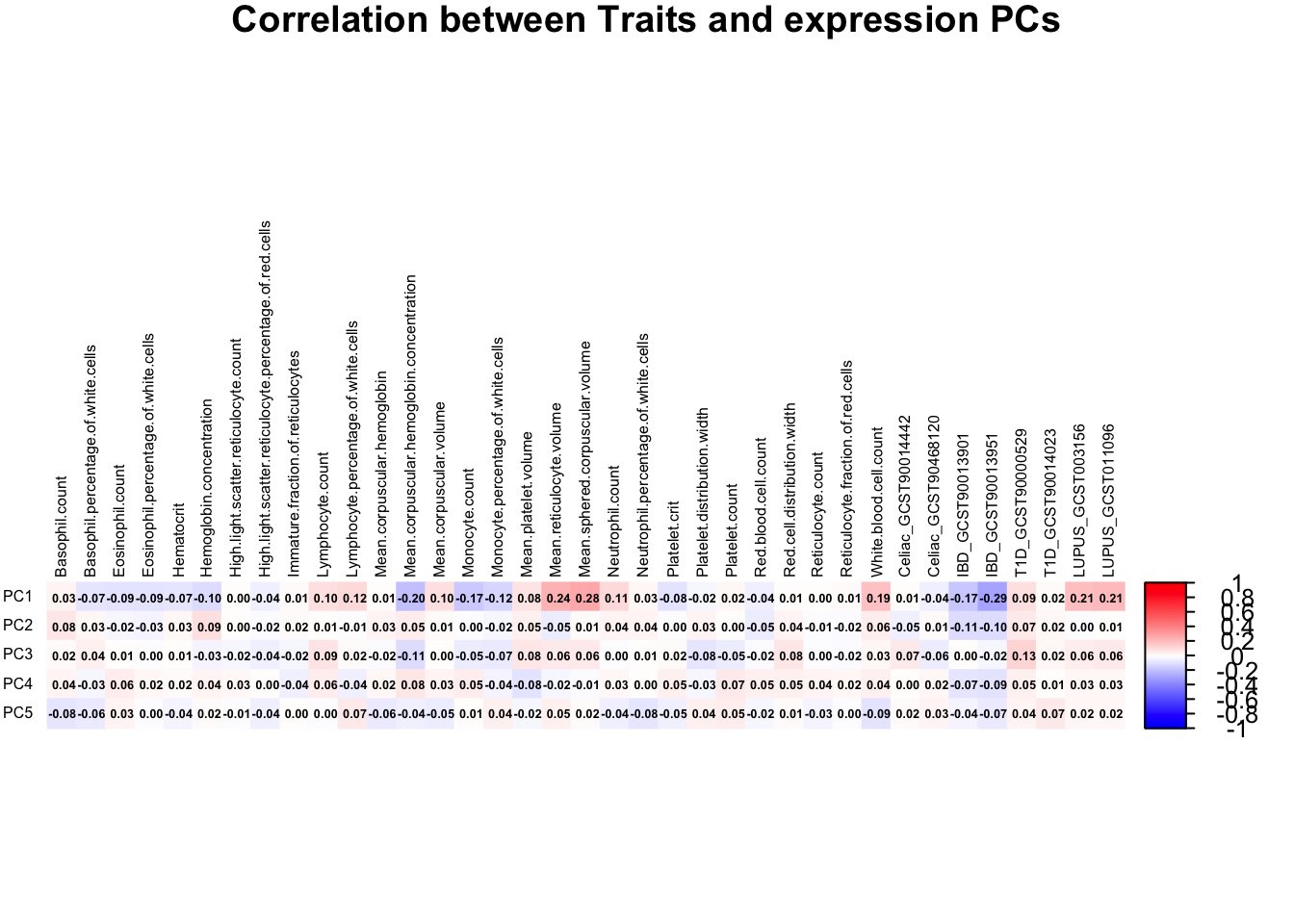
Correlation between PRS & expression PCs (whole blood)

# load prs & pcs
metadata_file <- "analysis/metadata.txt"
metadata <- read.csv(metadata_file, header = T, sep = "\t", stringsAsFactors = T)
metadata$sex <- as.factor(metadata$sex)

traits <- metadata[, 7:43]
pc <- metadata[, c(1:5)]

# Calculate the correlation between each trait and each PC
correlation_matrix <- cor(traits, pc)
range(correlation_matrix)

[1] -0.2850667  0.2787222

correlation_matrix <- t(correlation_matrix)

# Create the heatmap using corrplot
corrplot(correlation_matrix, method = "color", 
         col = colorRampPalette(c("blue", "white", "red"))(200), # color palette
         addCoef.col = "black", # Add correlation coefficients to the plot
         number.cex = 0.4, # Adjust the font size of the numbers
         tl.col = "black", # text label color
         tl.srt = 90, # rotate text labels
         tl.cex = 0.5, 
         title = "Correlation between Traits and expression PCs", 
         mar = c(0, 0, 1, 0)
)

Version	Author	Date
2b73cc3	ElisaChen	2025-05-13
c4ece77	ElisaChen	2025-04-30

Perform DESeq2 differential expression analysis for each trait

Model 1: expression ~ PRS + sex + expression PCs

Continuous PRS:

# Load the gene expression data
gene_expr_file <- "data/gene_reads_2017-06-05_v8_whole_blood.gct"
raw_count_df <- fread(gene_expr_file, header = TRUE, sep = "\t", drop = "id")

# load protein_coding list
protein_coding <- fread("data/protein-coding_gene.txt", sep = "\t")
protein_coding <- protein_coding[, c("symbol", "ensembl_gene_id")]

# keep only protein-coding genes
raw_count_df <- raw_count_df[raw_count_df$Description %in% protein_coding$symbol, ]

id <- raw_count_df$Name
raw_count <- raw_count_df[, -c(1:2)]

# modify GTEx sample names matching names used in PRS data
colnames(raw_count) <- sub("^(GTEX-[^-.]+).*", "\\1", colnames(raw_count))

matching_samples <- intersect(rownames(metadata), colnames(raw_count))
final_count <- raw_count[ , ..matching_samples]

# prefilter: keep only rows that have a count of at least 10
keep_genes <- rowSums(final_count >= 10) > 0
final_count <- final_count[keep_genes, ]
id <- id[keep_genes]
dim(final_count)

# Loop through each trait and run DESeq2
for (trait in colnames(traits)) {
  
  # Standardize PRS for the current trait
  prs_trait <- traits[,trait]
  prs_trait <- scale(prs_trait) # Standardize PRS to mean = 0, sd = 1
    
  # Add the standardized PRS to the metadata for continuous trait
  metadata[,trait] <- prs_trait
  
  # Create the DESeqDataSet for the current trait
  dds <- DESeqDataSetFromMatrix(
    countData = as.matrix(final_count),  # Raw counts
    colData = metadata[, c(1:6, which(colnames(metadata) == trait))],
    design = as.formula(paste("~ PC1 + PC2 + PC3 + PC4 + PC5 + sex +", trait))
  )
  rownames(dds) <- id
  
  # Run DESeq2 analysis
  dds <- DESeq(dds, parallel = TRUE, BPPARAM = MulticoreParam(4))
  
  # Get the results for the current trait
  res <- results(dds)
  
  # Save the results to a file
  write.csv(res, paste0("differential_expression_", trait, "_results.csv"))
  
  # print a summary of the results
  print(paste("Results for trait:", trait))
  print(summary(res))
  
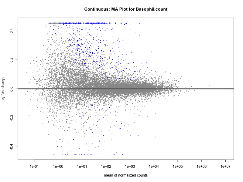
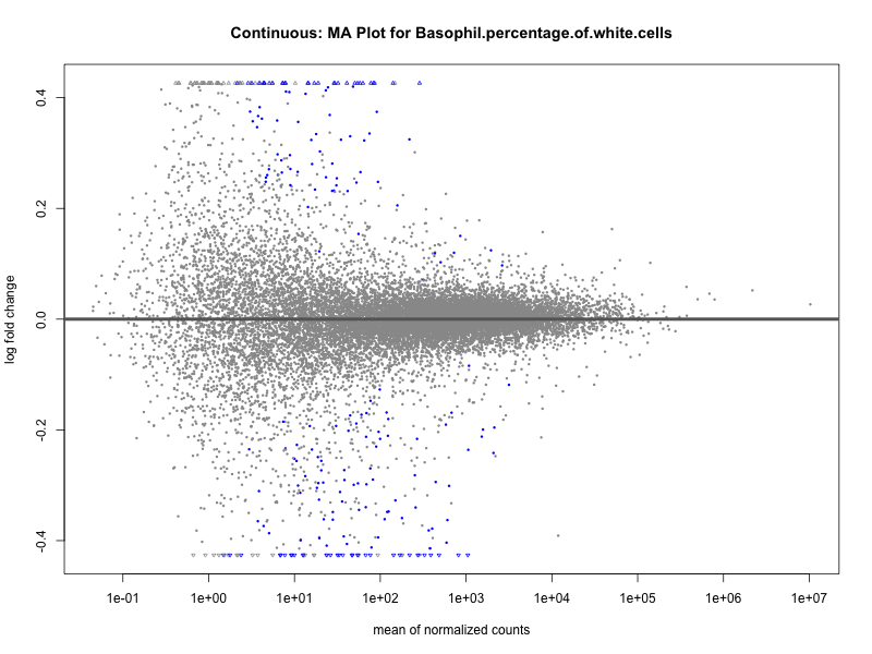
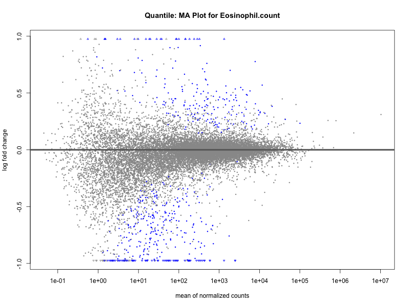
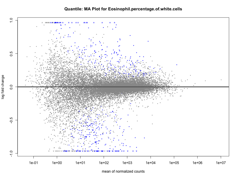
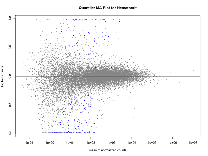
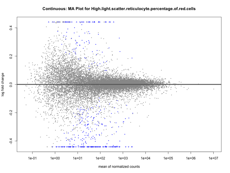
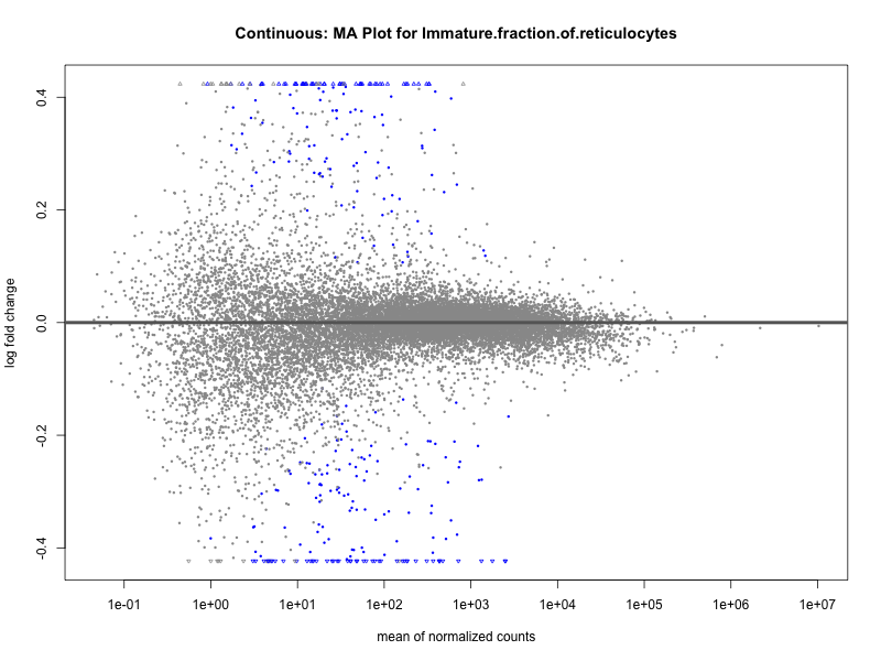
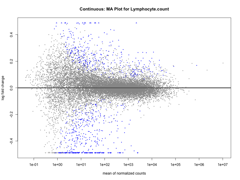
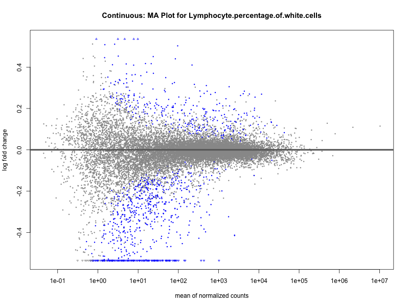
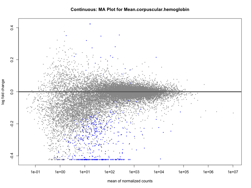
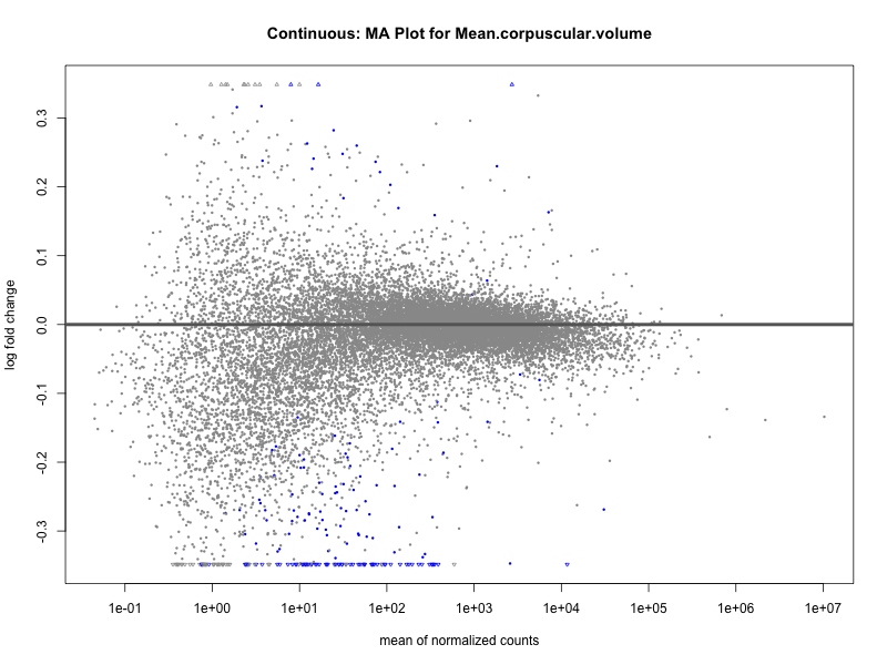
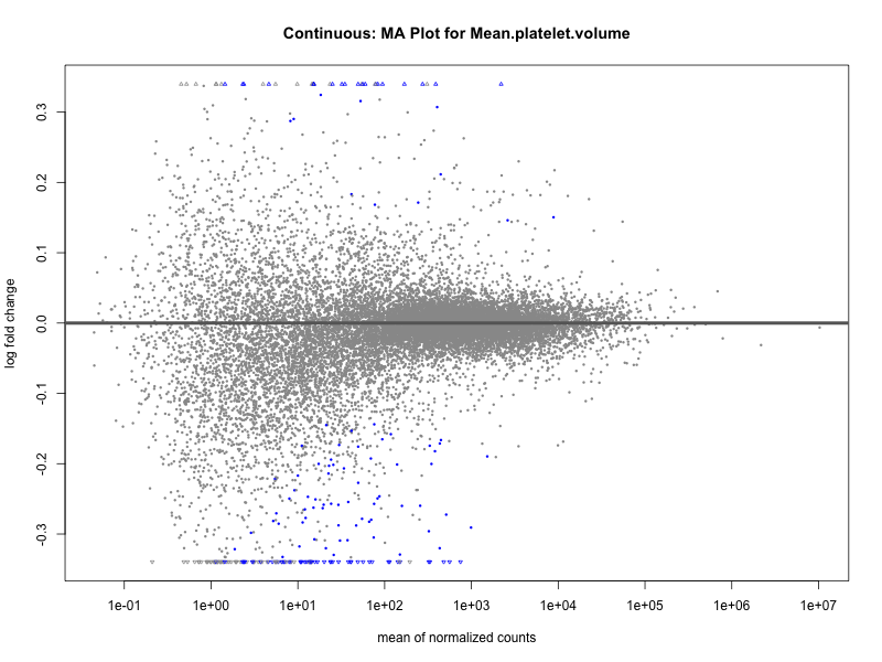
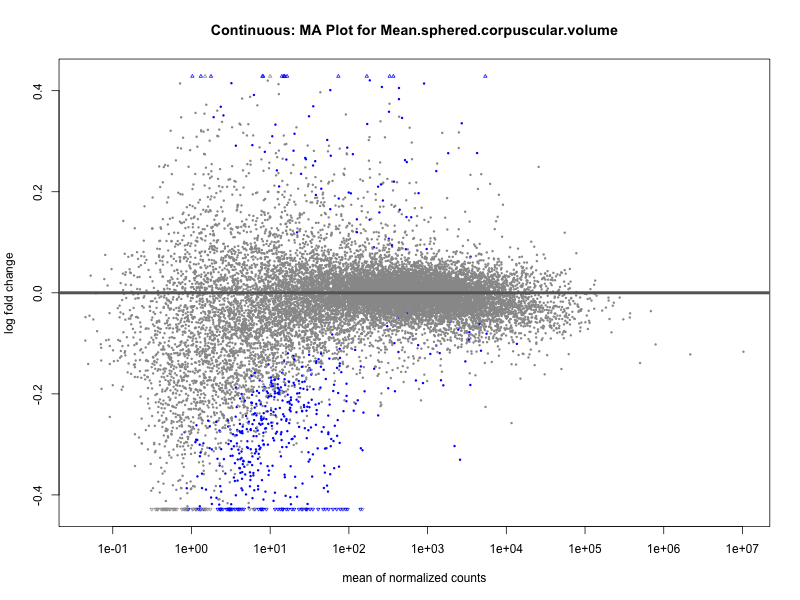
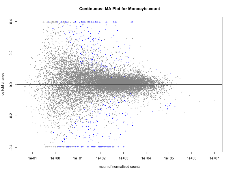
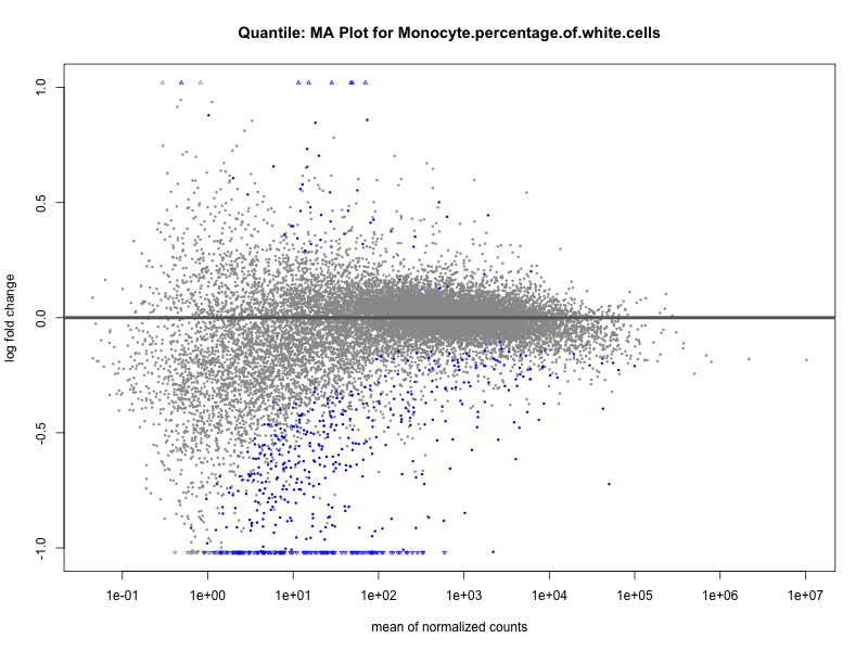
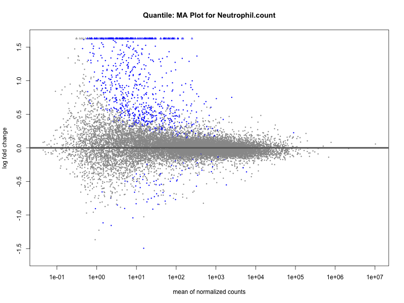
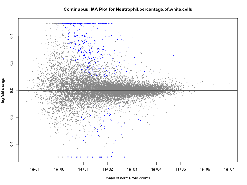
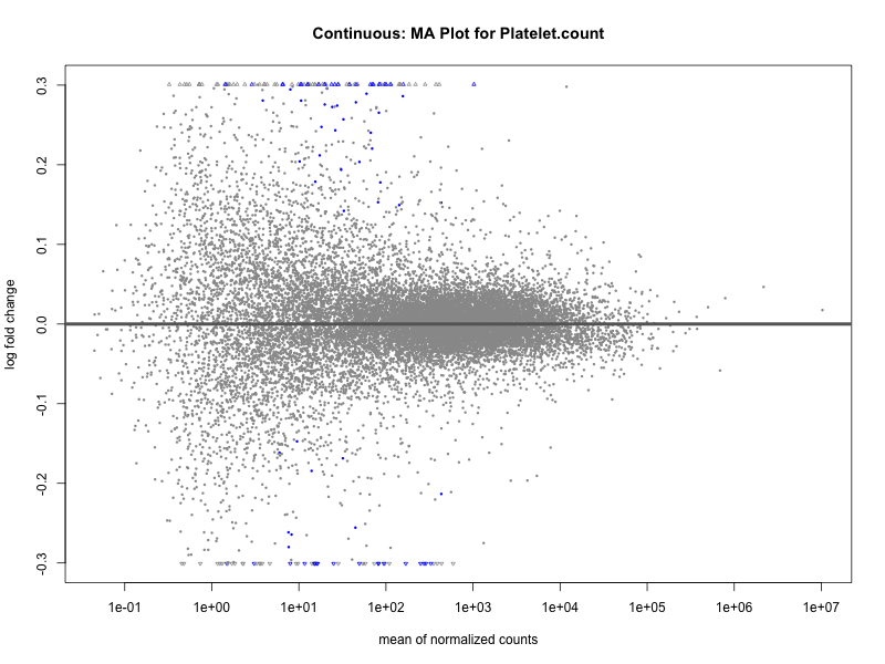
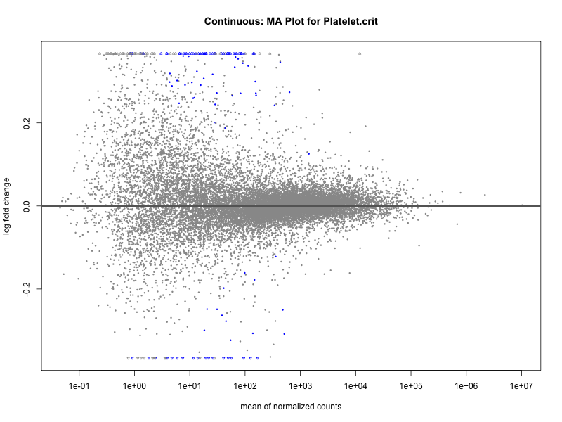
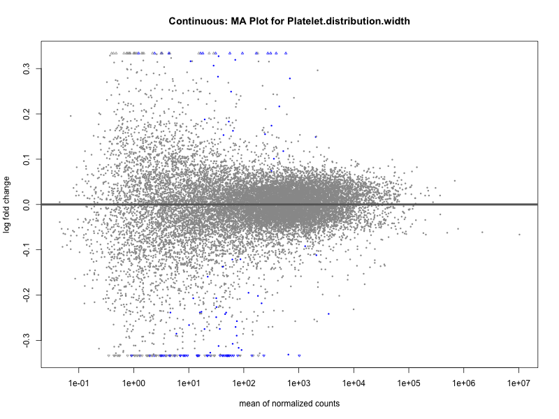
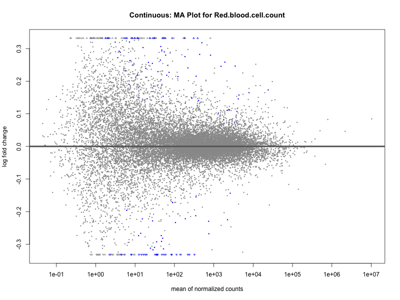
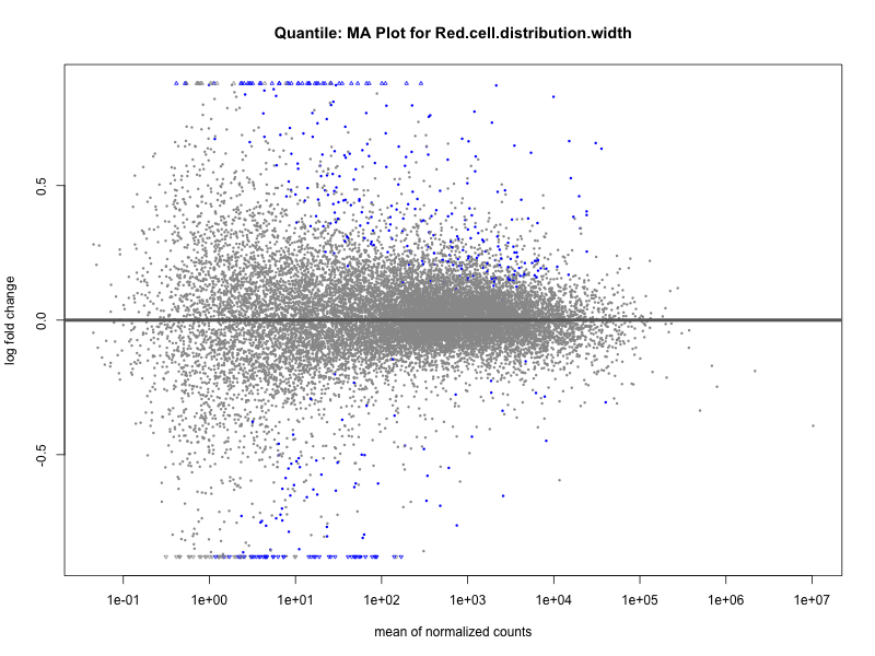
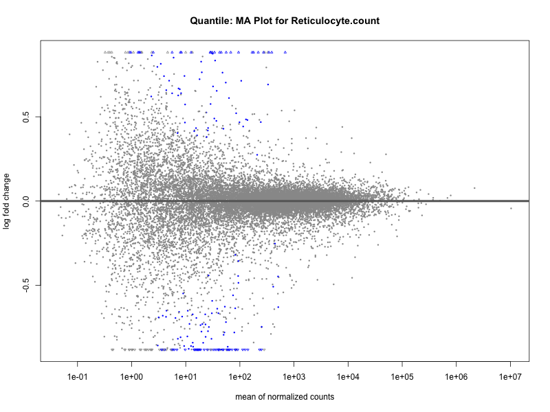
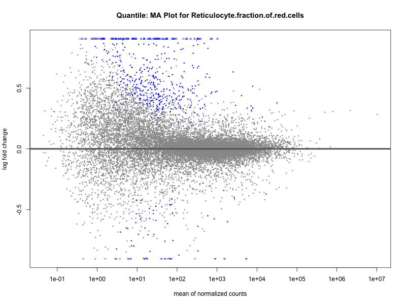
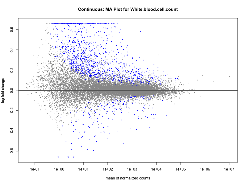
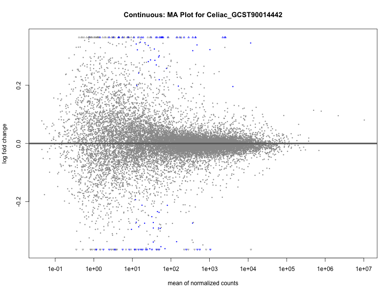
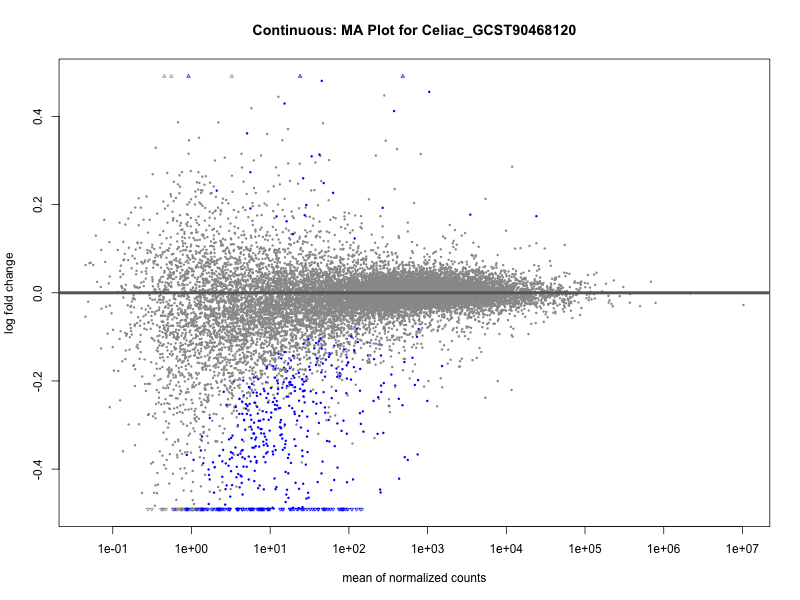
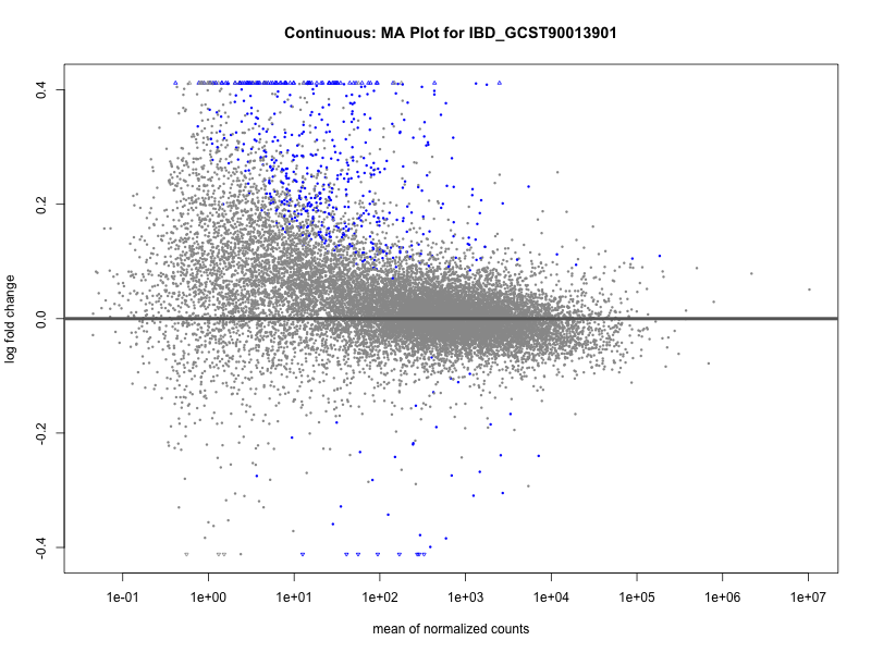
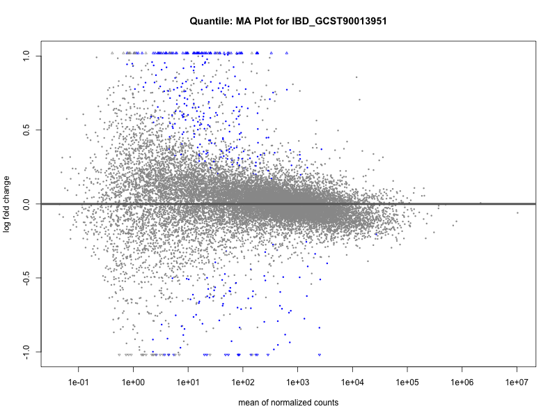
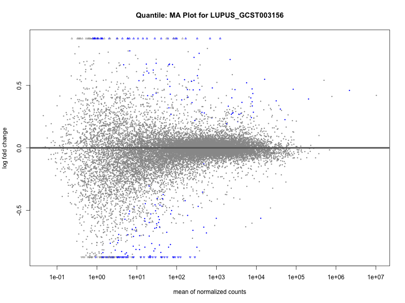
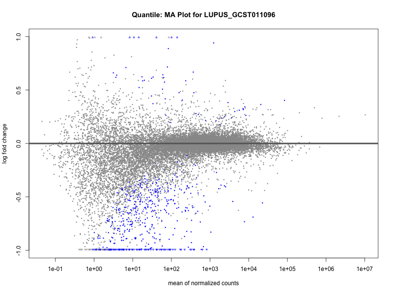
  # plot the MA-plot for the current trait
  png(paste0("ma_plot_", trait, ".png"), width = 800, height = 600)
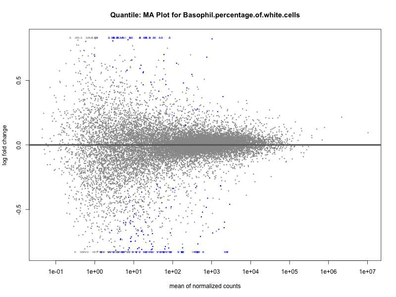
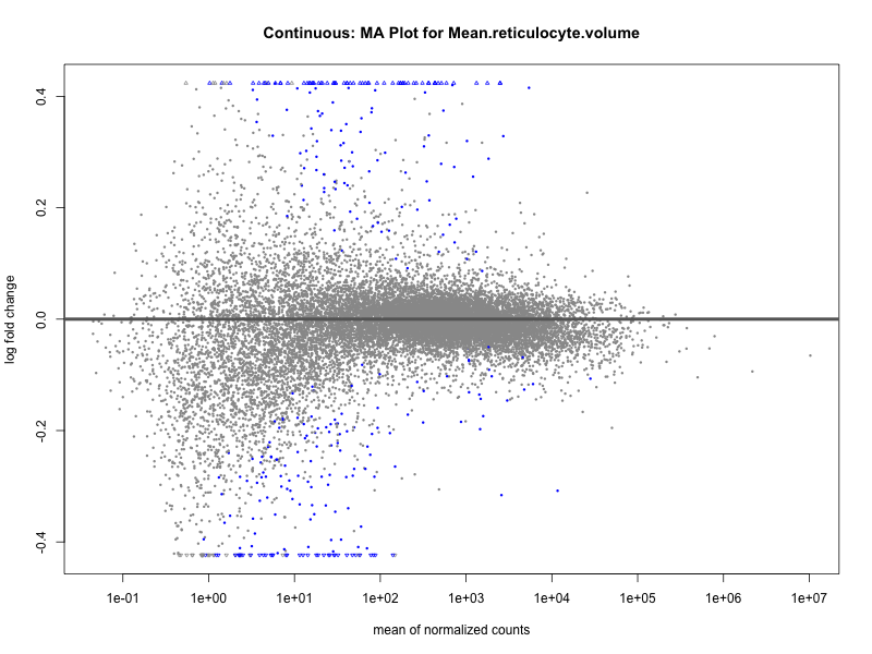
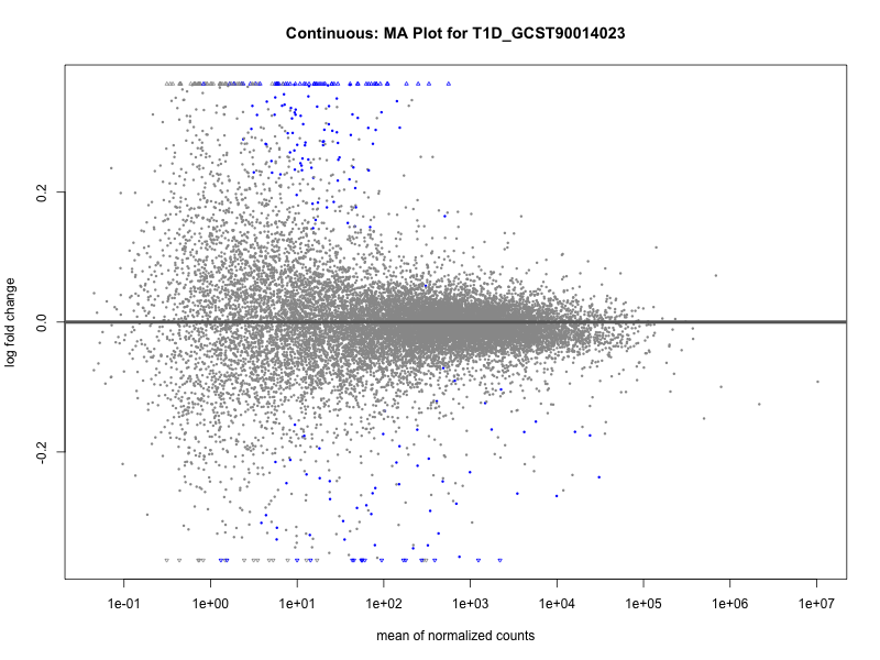
  plotMA(res, main = paste("Continuous: MA Plot for", trait))
  dev.off()
  
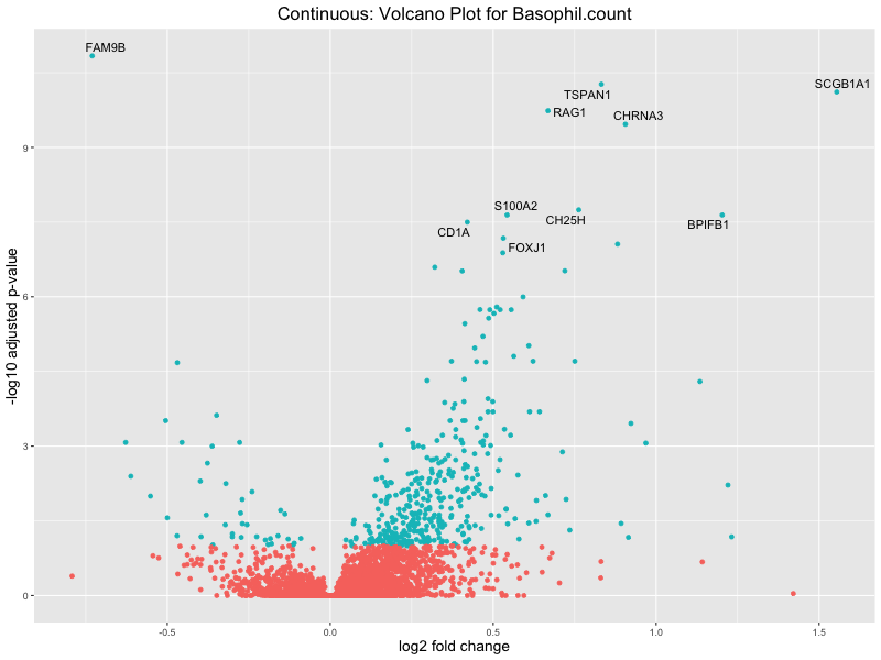
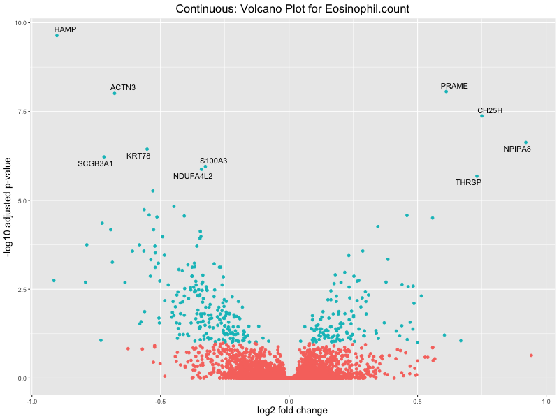
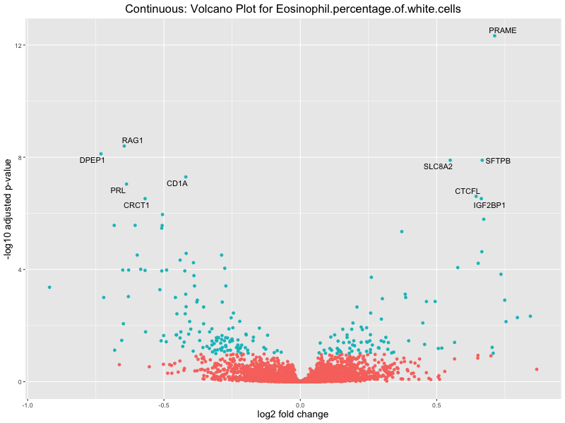
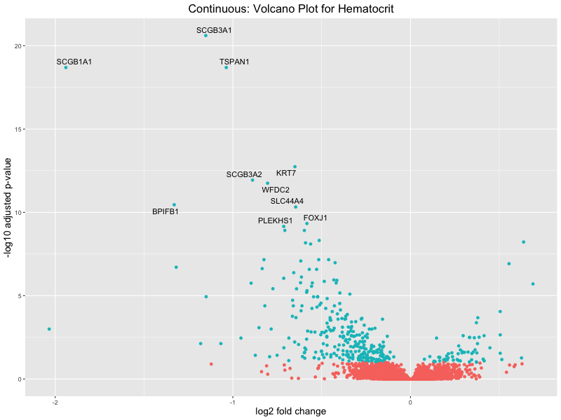
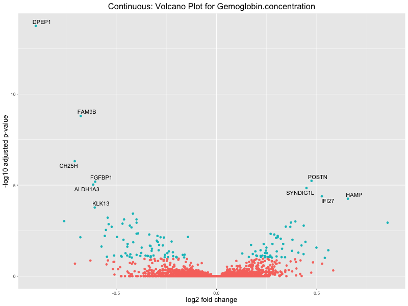
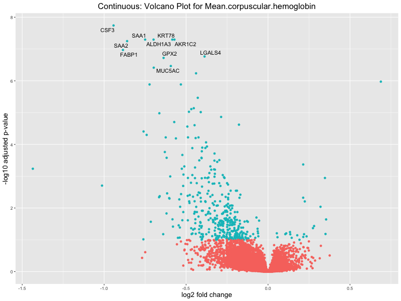
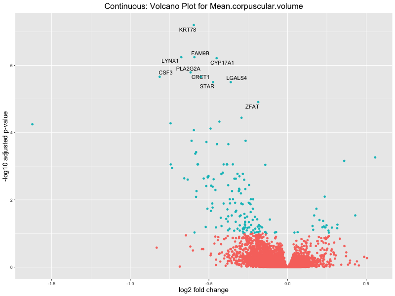
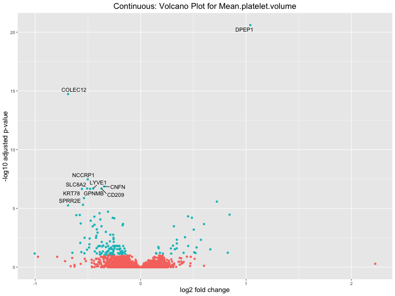
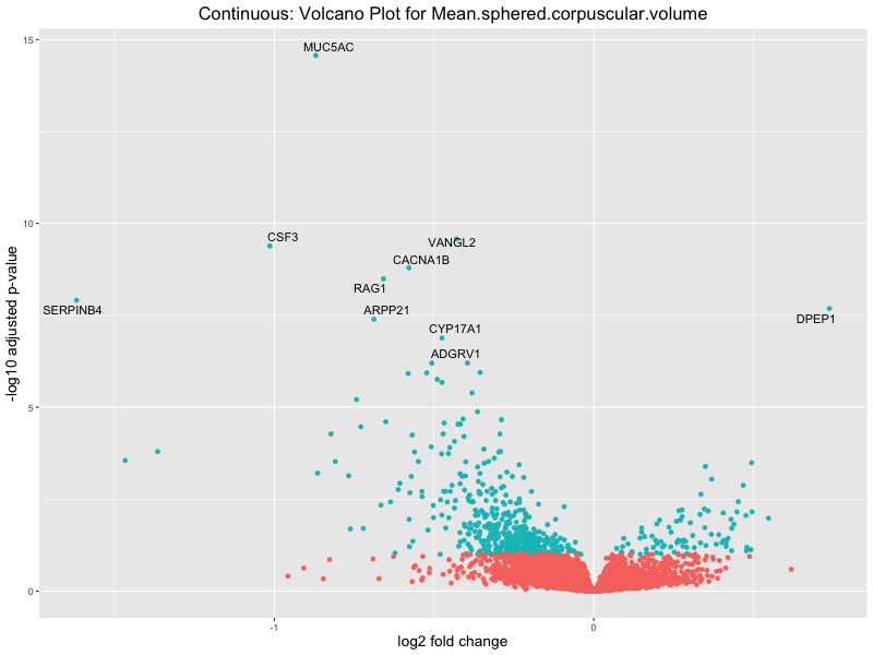
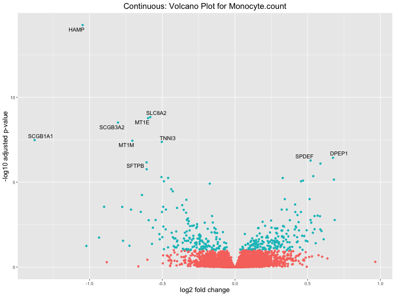
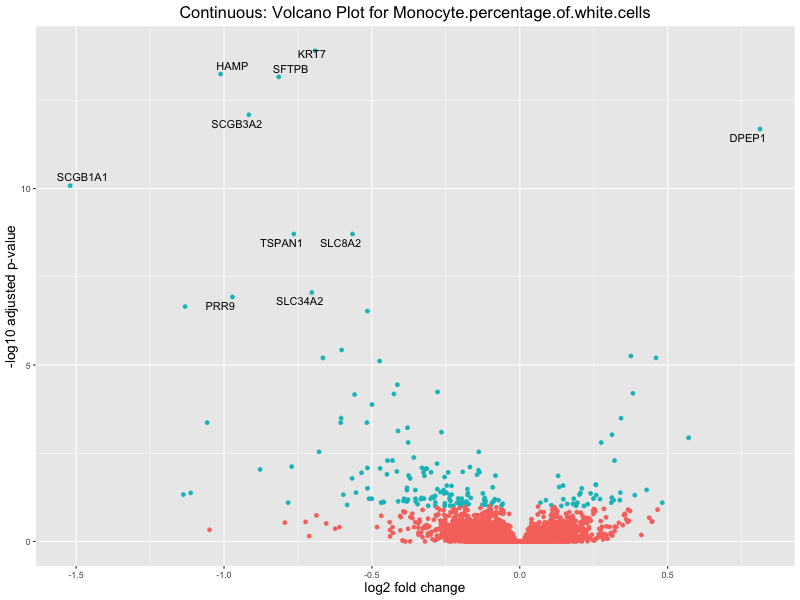
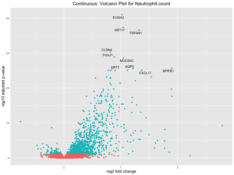
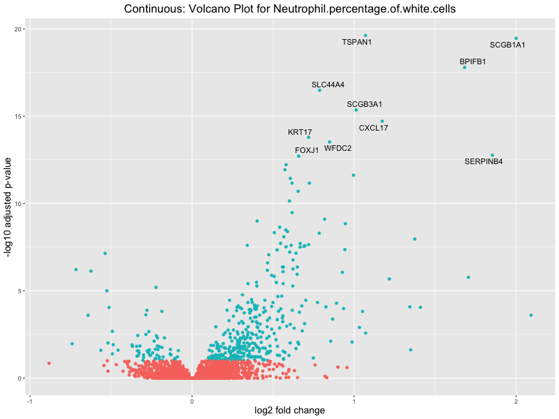
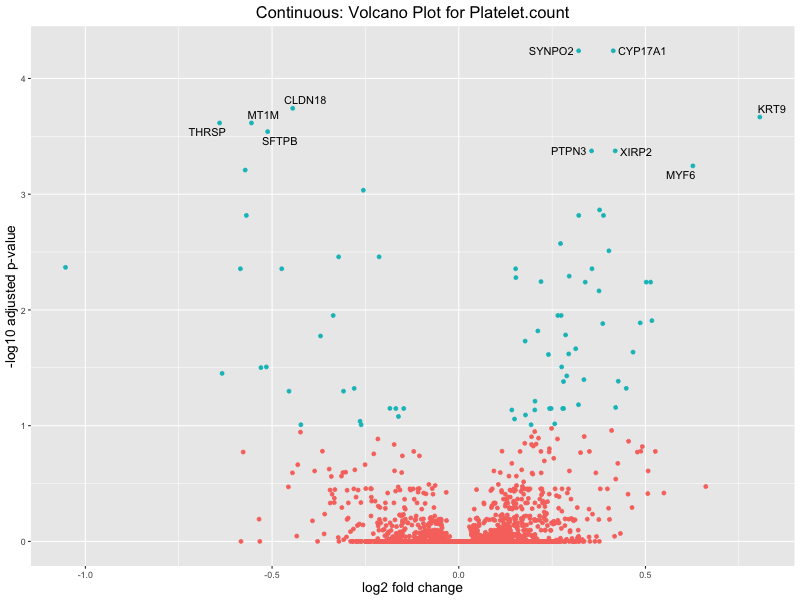
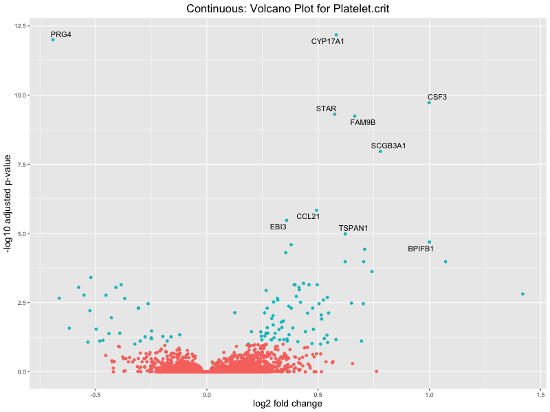
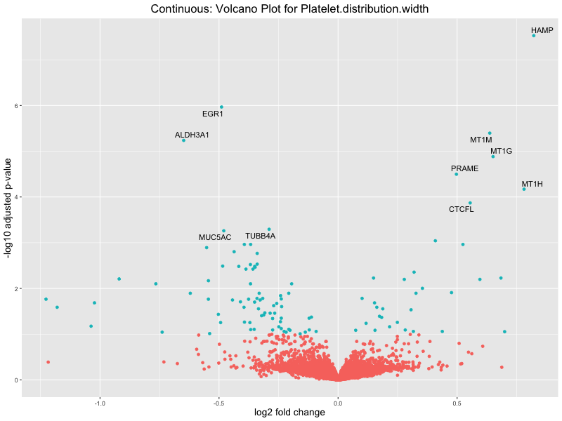
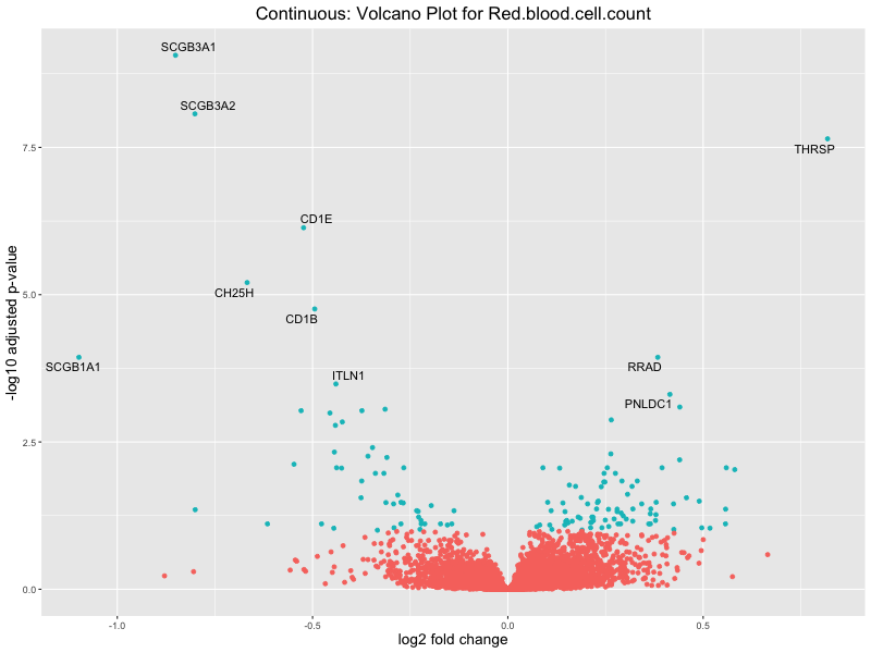
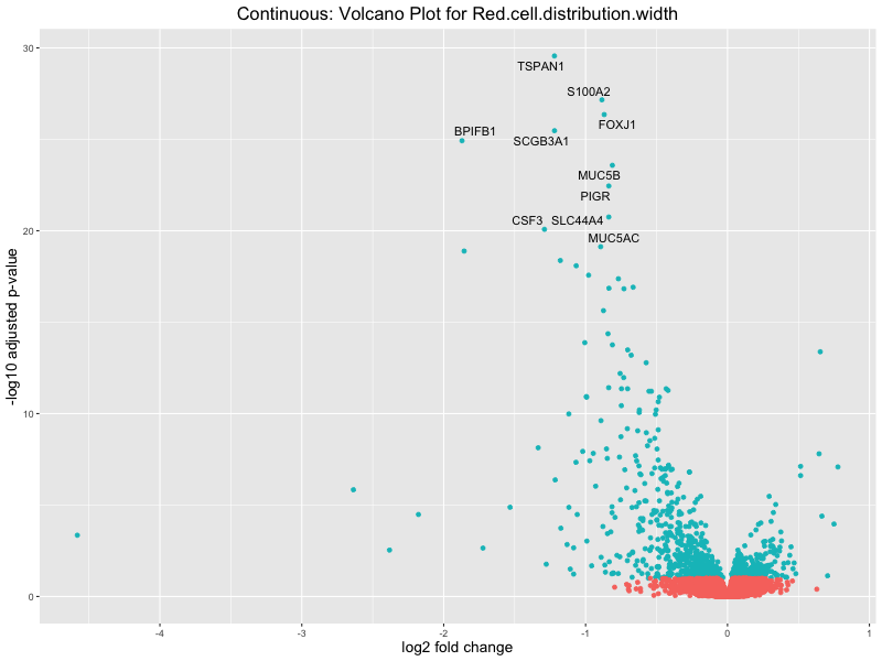
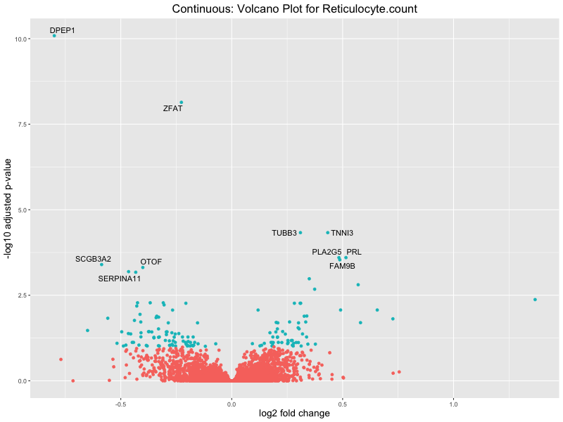
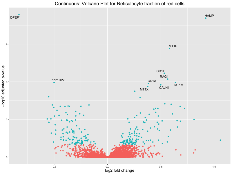
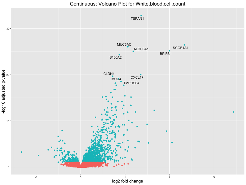
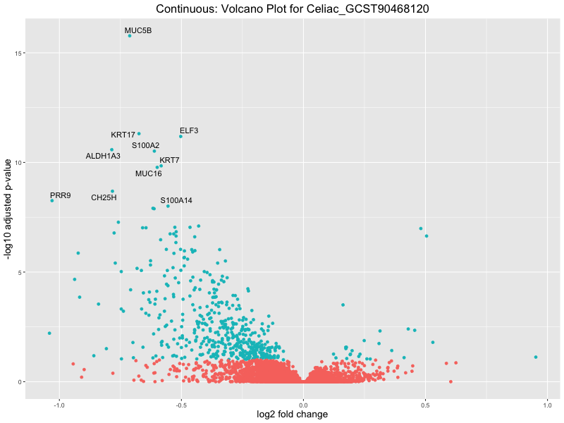
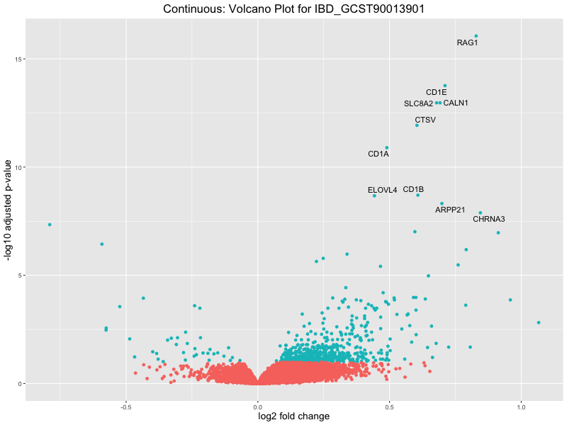
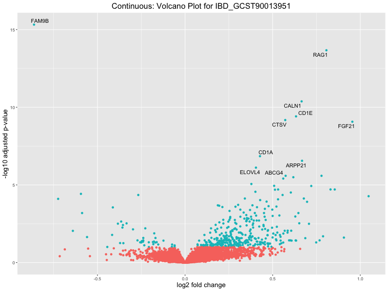
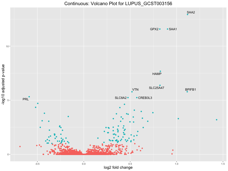
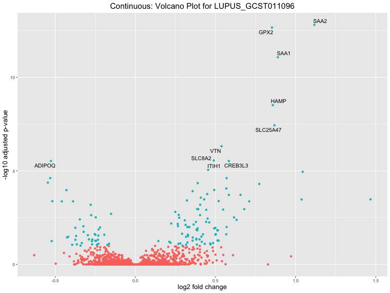
  # volcano plot
  res_tableOE <- as.data.frame(res)
  res_tableOE$gene_name <- raw_count_df$Description[keep_genes]
  res_tableOE <- mutate(res_tableOE, threshold_OE = padj < 0.1)
  res_tableOE <- res_tableOE %>% arrange(padj) %>% mutate(genelabels = "")
  res_tableOE$genelabels[1:10] <- res_tableOE$gene_name[1:10]
  
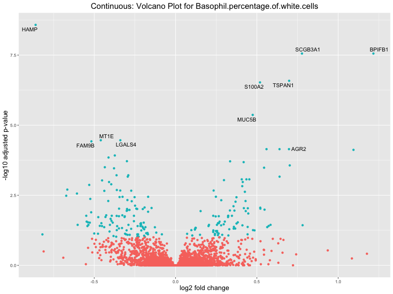
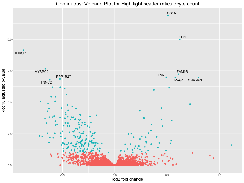
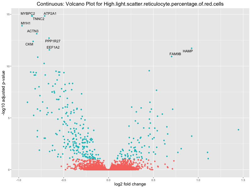
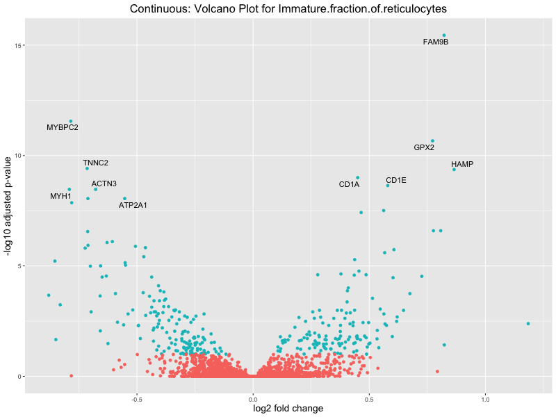
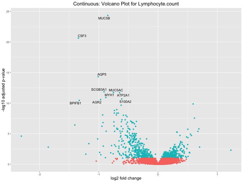
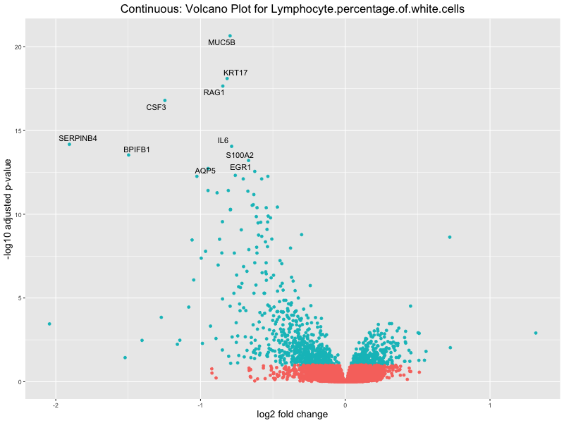
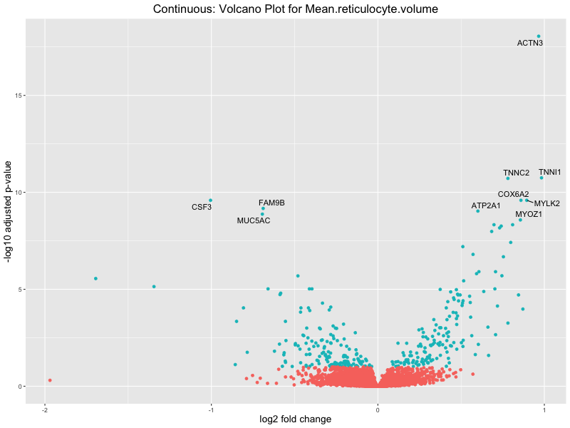
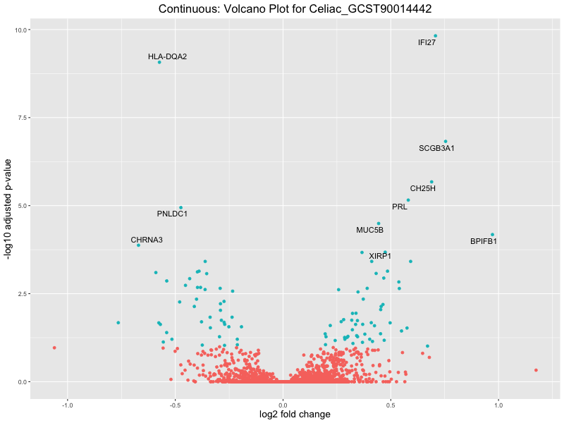
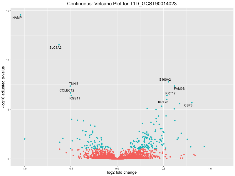
  volcano_plot <- ggplot(res_tableOE, aes(x = log2FoldChange, y = -log10(padj))) +
    geom_point(aes(colour = threshold_OE)) +
    geom_text_repel(aes(label = genelabels)) +
    ggtitle(paste("Continuous: Volcano Plot for", trait)) +
    xlab("log2 fold change") + 
    ylab("-log10 adjusted p-value") +
    theme(legend.position = "none",
          plot.title = element_text(size = rel(1.5), hjust = 0.5),
          axis.title = element_text(size = rel(1.25)))
  
  # Save the volcano plot
  png(paste0("volcano_plot_", trait, ".png"), width = 800, height = 600)
  print(volcano_plot)
  dev.off()
}

Quantile PRS:

metadata_file <- "analysis/metadata_quantile.txt"
metadata <- read.csv(metadata_file, header = T, sep = "\t", stringsAsFactors = T)
metadata$sex <- as.factor(metadata$sex)

traits <- metadata[, 7:43]

# Loop through each trait and run DESeq2
for (trait in colnames(traits)) {
  
  # Create the DESeqDataSet for the current trait
  dds <- DESeqDataSetFromMatrix(
    countData = as.matrix(final_count),  # Raw counts
    colData = metadata[, c(1:6, which(colnames(metadata) == trait))],
    design = as.formula(paste("~ PC1 + PC2 + PC3 + PC4 + PC5 + sex +", trait))
  )
  rownames(dds) <- id
  
  # Run DESeq2 analysis
  dds <- DESeq(dds, parallel = TRUE, BPPARAM = MulticoreParam(4))
  
  # Get the results for the current trait
  res <- results(dds)
  
  # Save the results to a file
  write.csv(res, paste0("differential_expression_", trait, "_quantile_results.csv"))
  
  # print a summary of the results
  print(paste("Results for trait:", trait))
  print(summary(res))
  
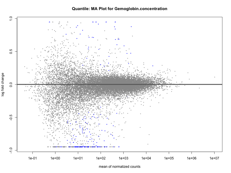
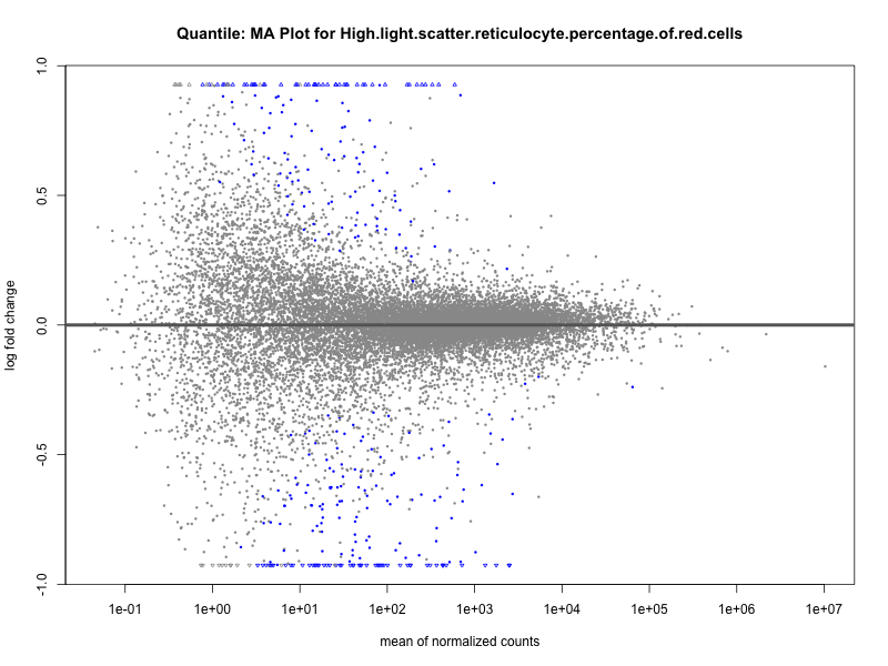
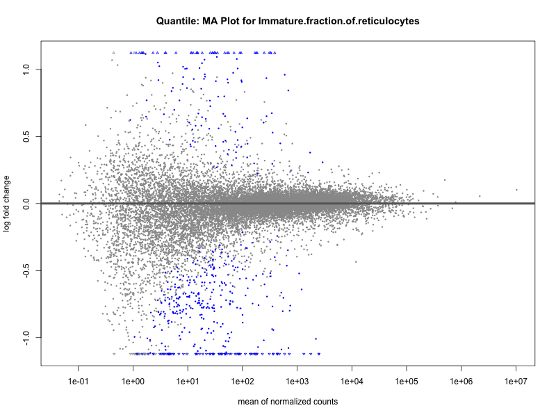
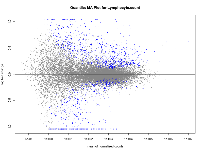
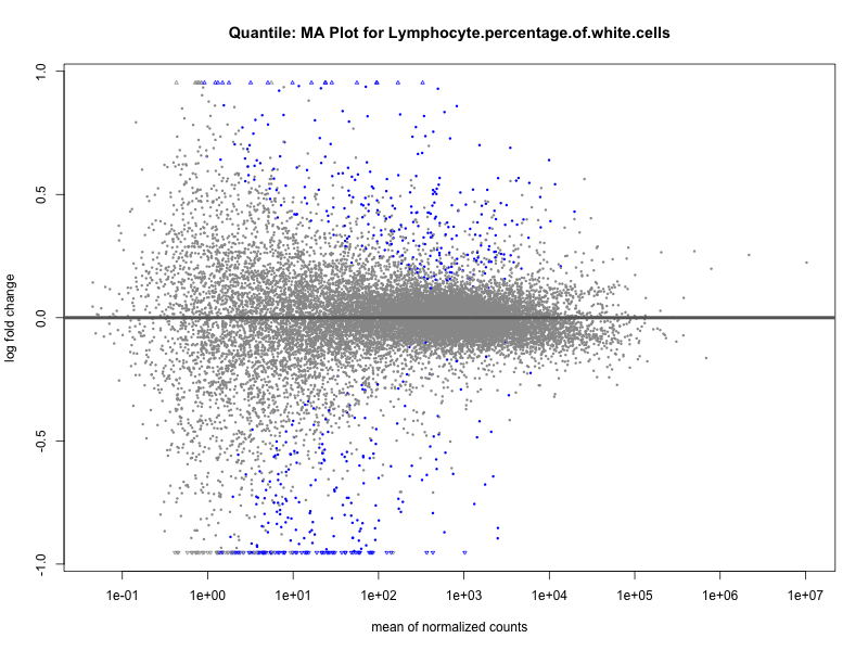
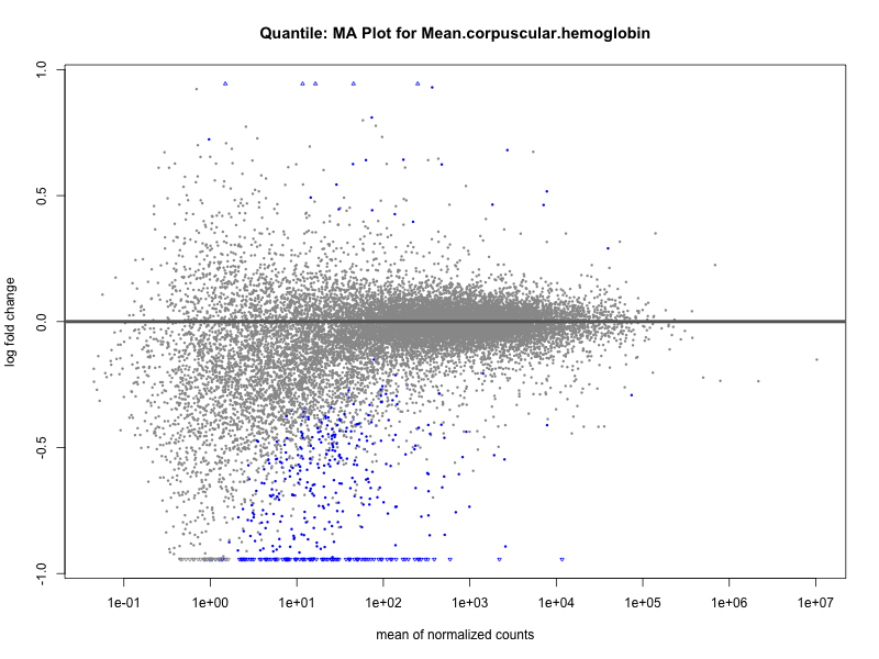
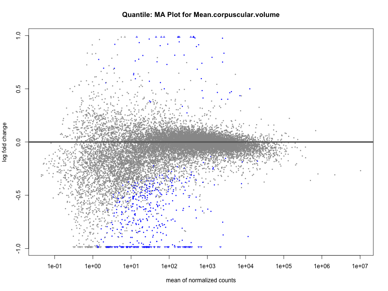
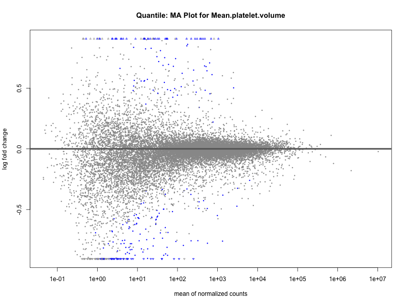
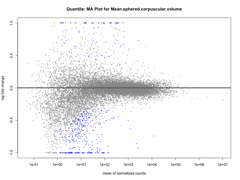
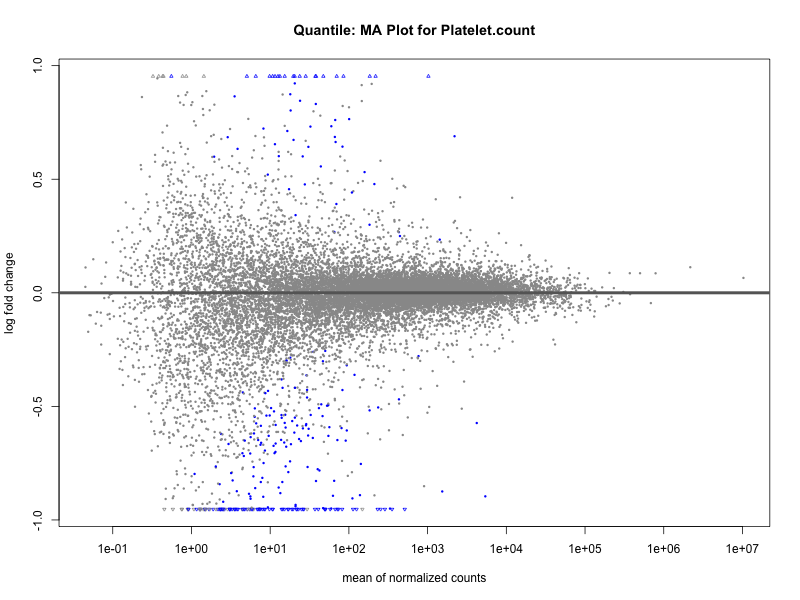
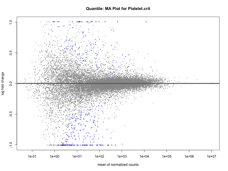
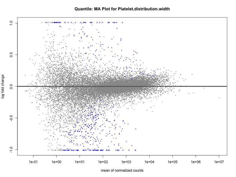
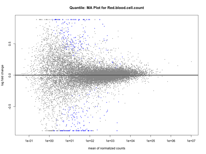
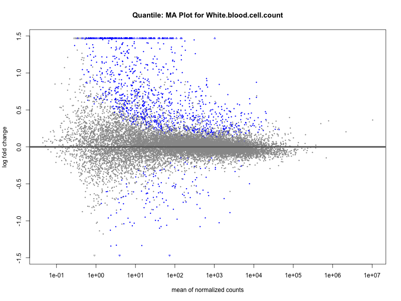
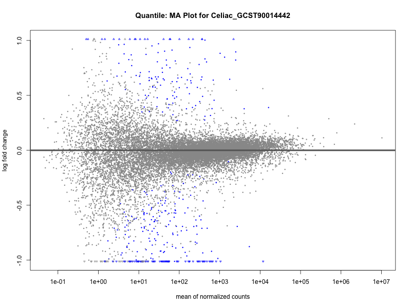
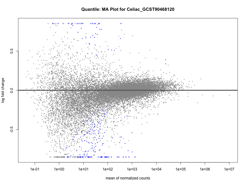
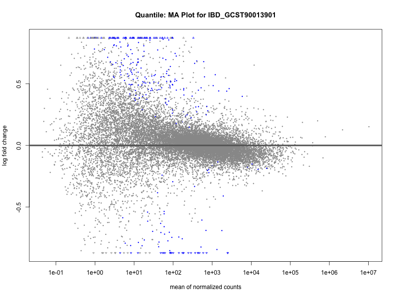
  # plot the MA-plot for the current trait
  png(paste0("ma_plot_quantile_", trait, ".png"), width = 800, height = 600)
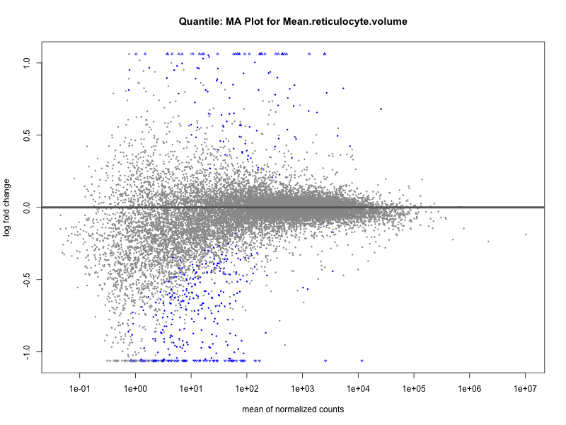
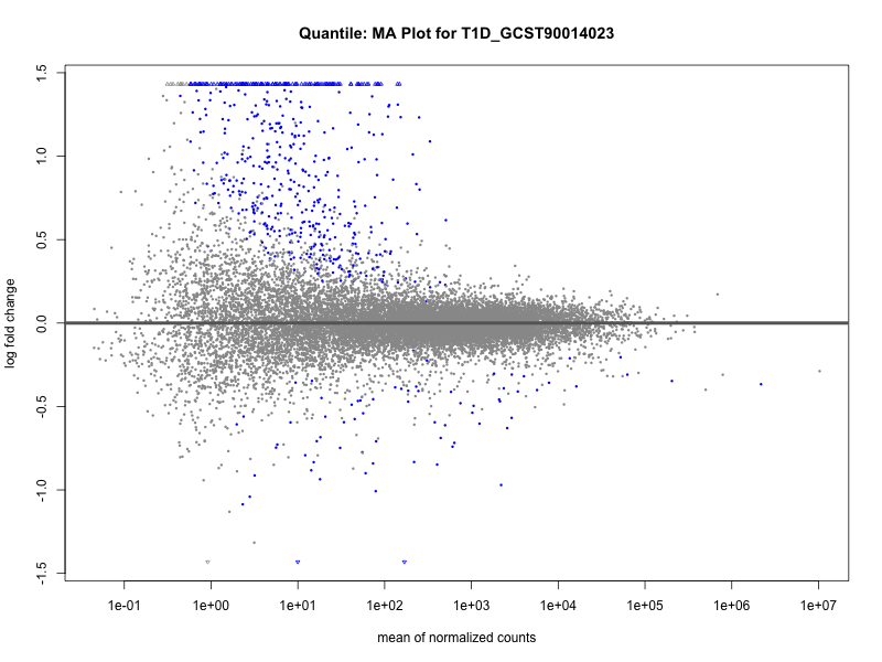
  plotMA(res, main = paste("Quantile: MA Plot for", trait))
  dev.off()
  
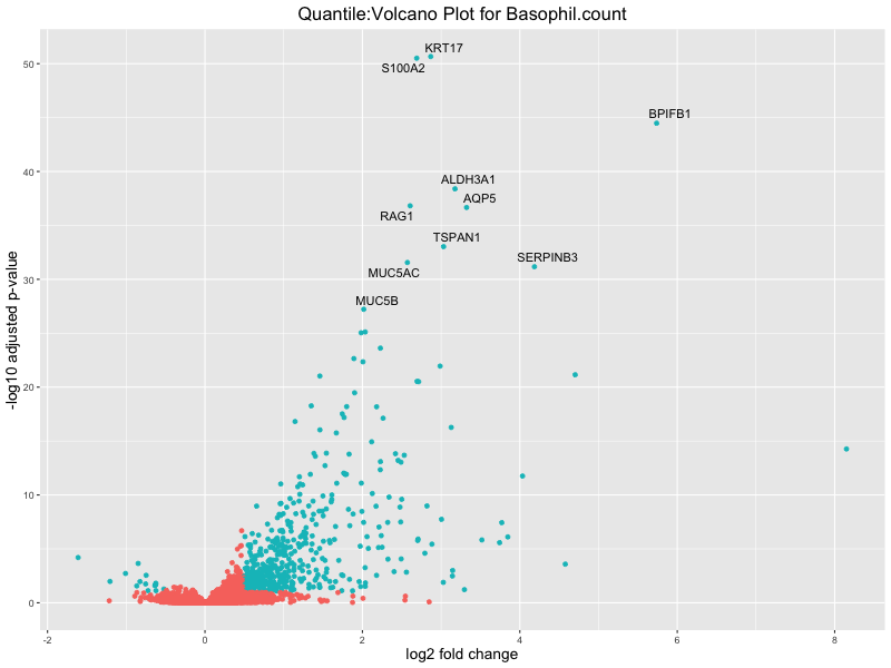
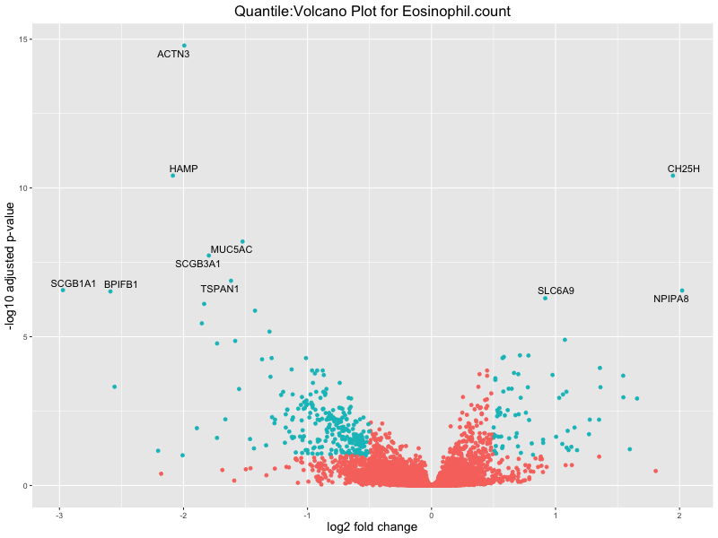
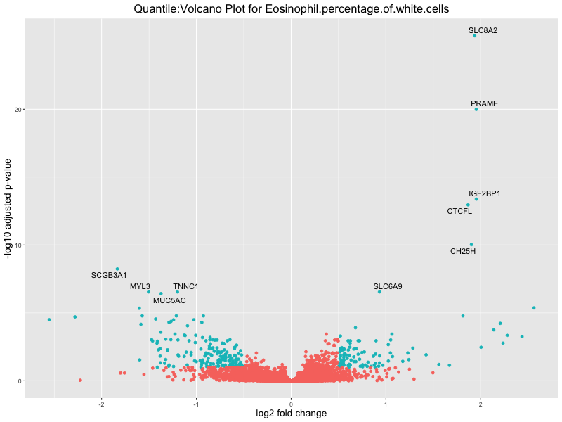
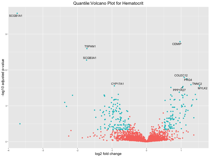
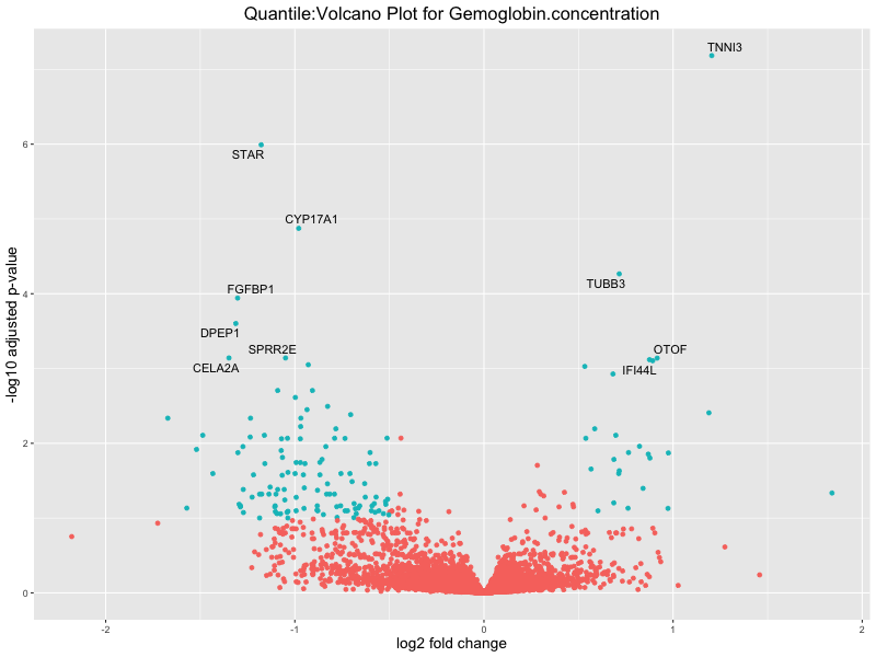
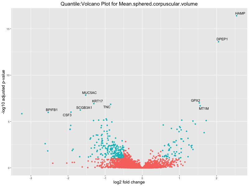
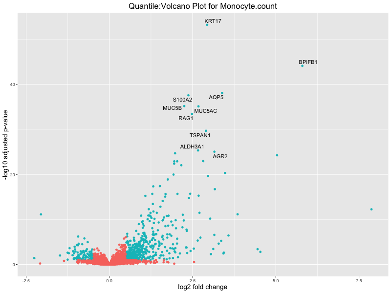
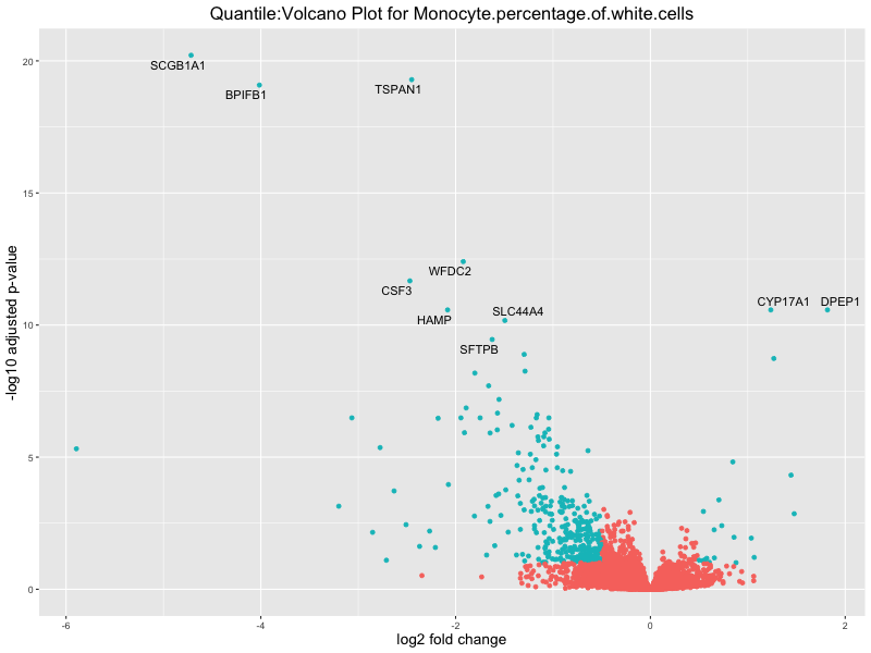
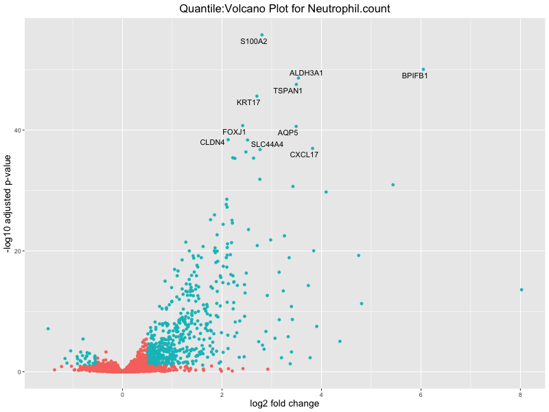
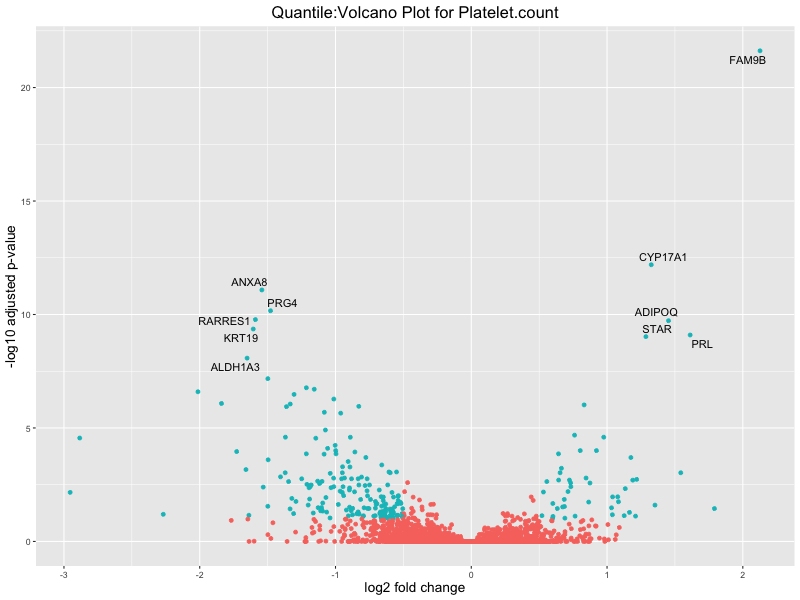
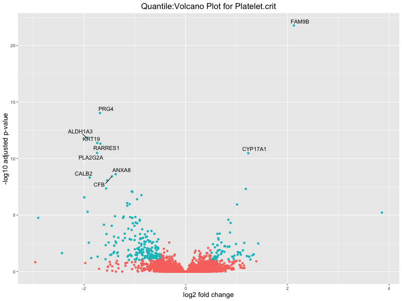
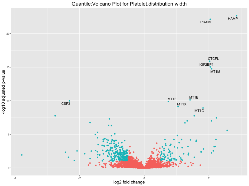
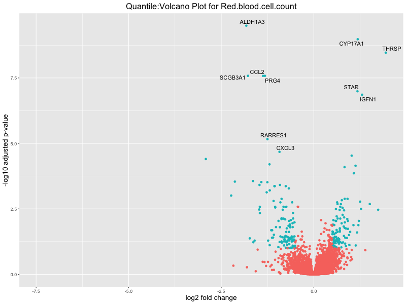
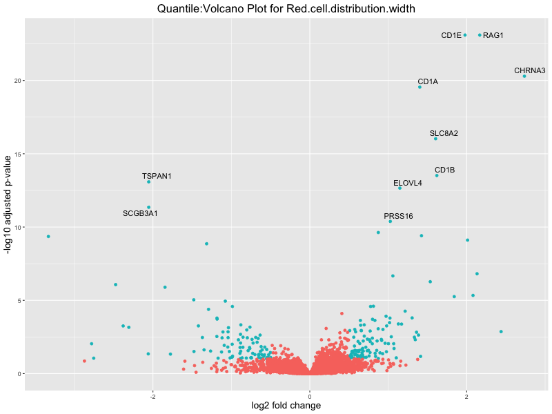
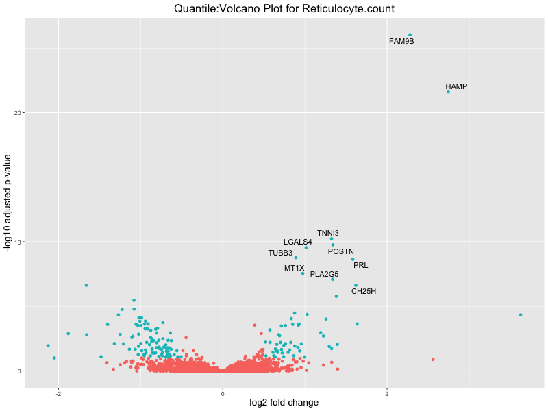
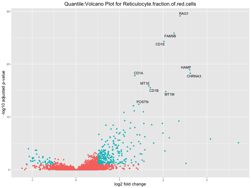
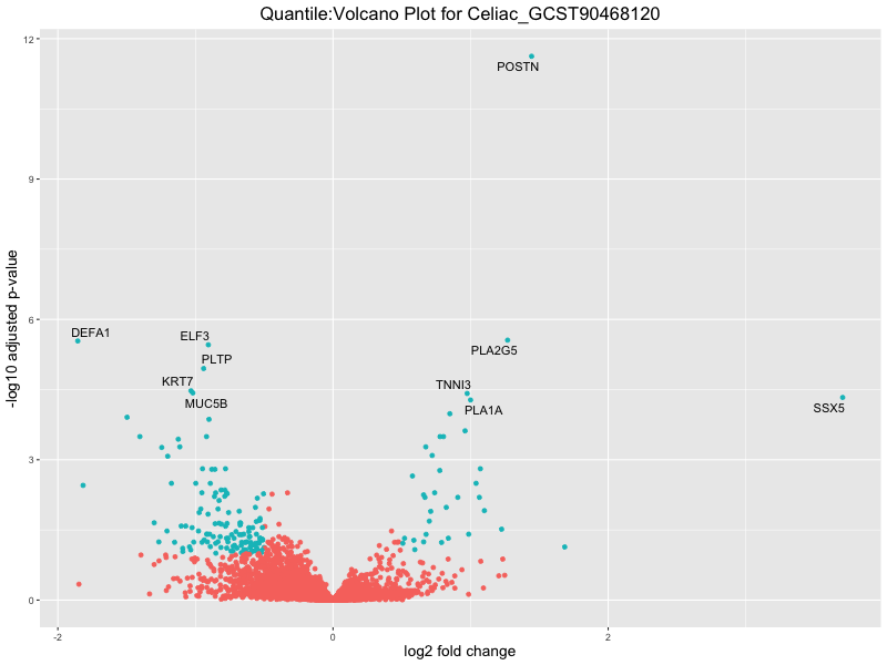
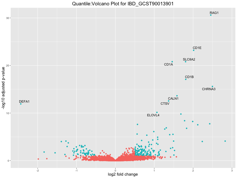
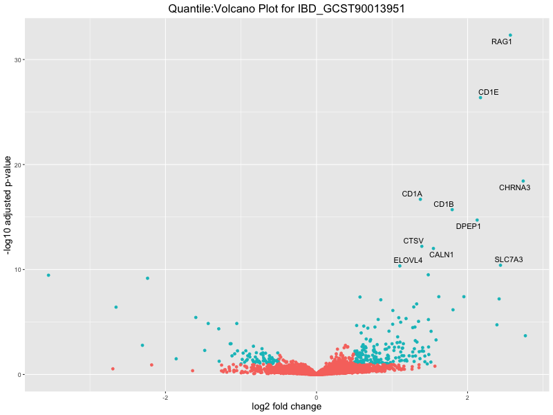
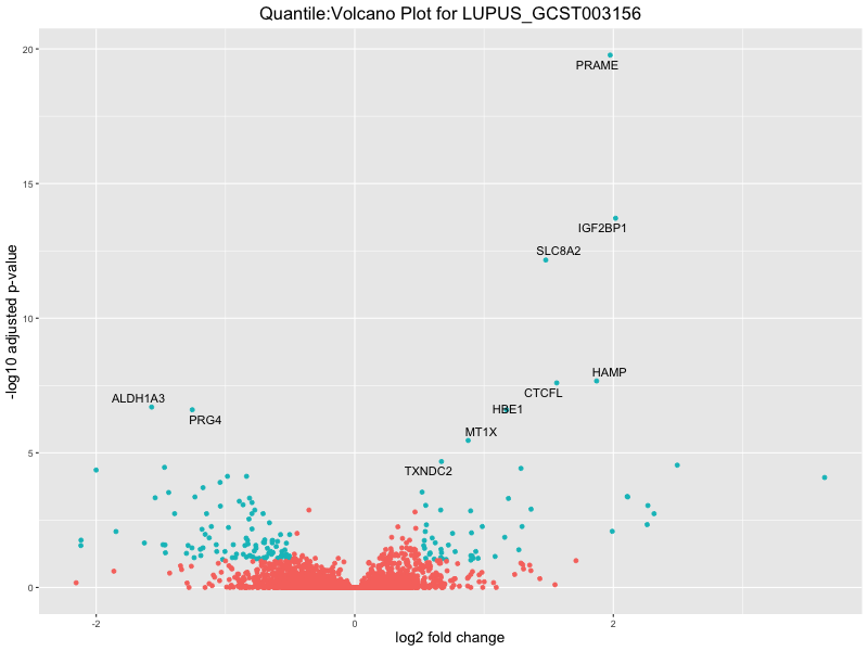
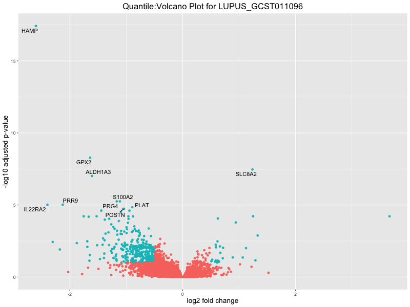
  # volcano plot
  res_tableOE <- as.data.frame(res)
  res_tableOE$gene_name <- raw_count_df$Description[keep_genes]
  res_tableOE <- mutate(res_tableOE, threshold_OE = padj < 0.1 & 
                          abs(log2FoldChange) >= 0.5)
  res_tableOE <- res_tableOE %>% arrange(padj) %>% mutate(genelabels = "")
  res_tableOE$genelabels[1:10] <- res_tableOE$gene_name[1:10]
  
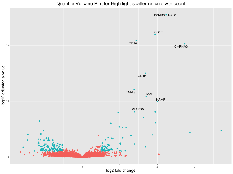
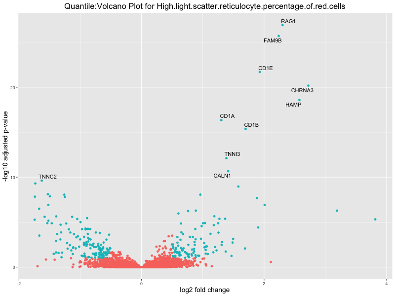
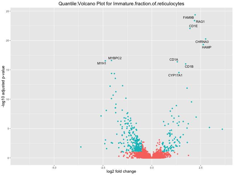
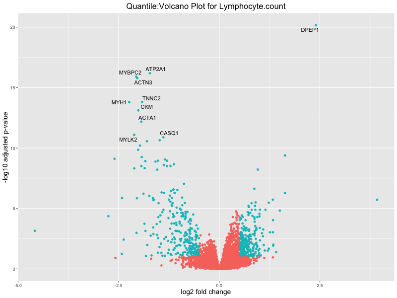
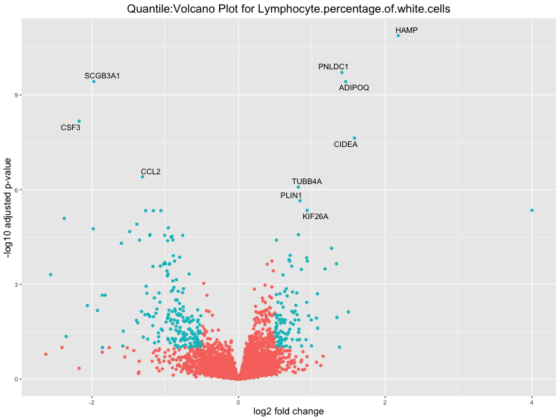
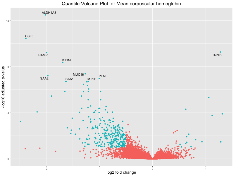
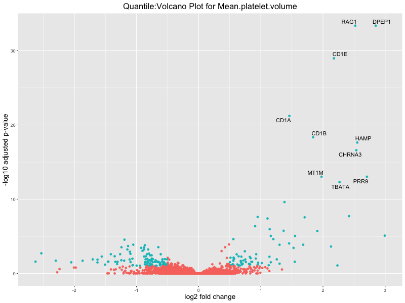
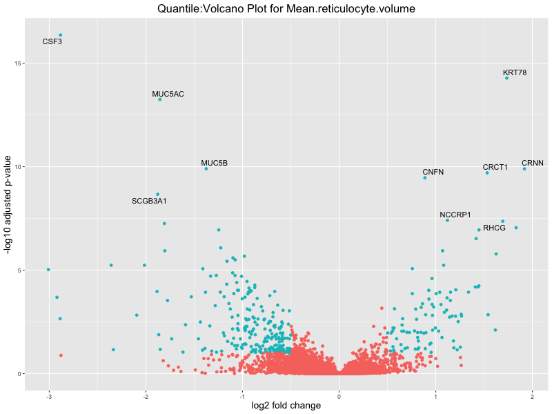
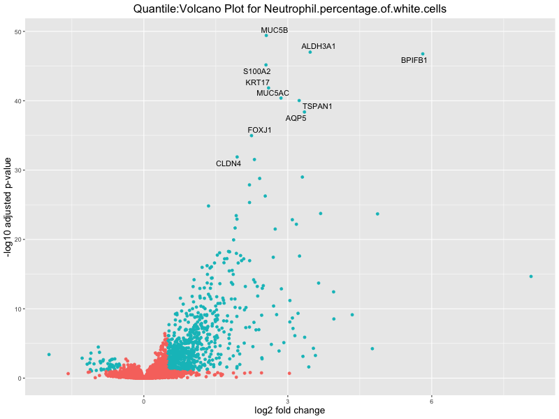
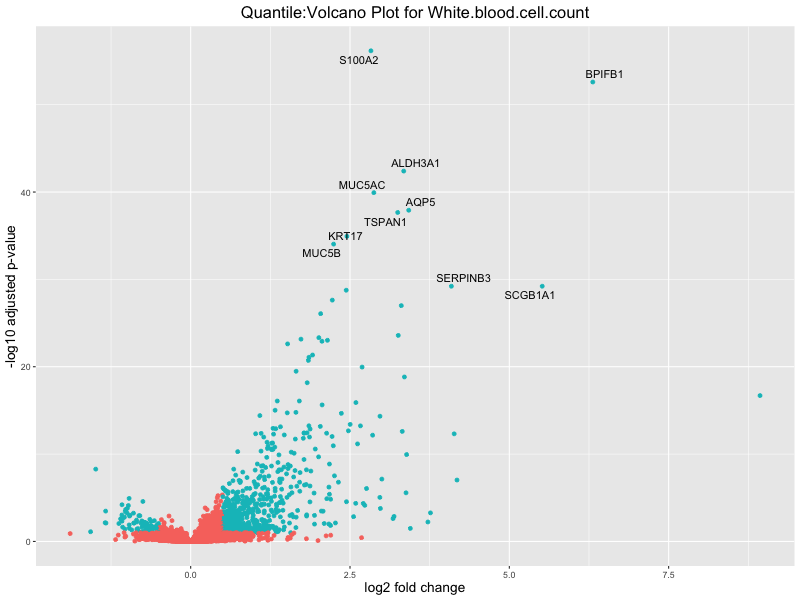
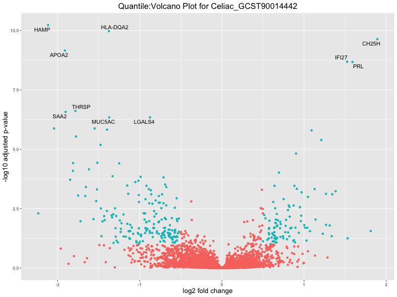
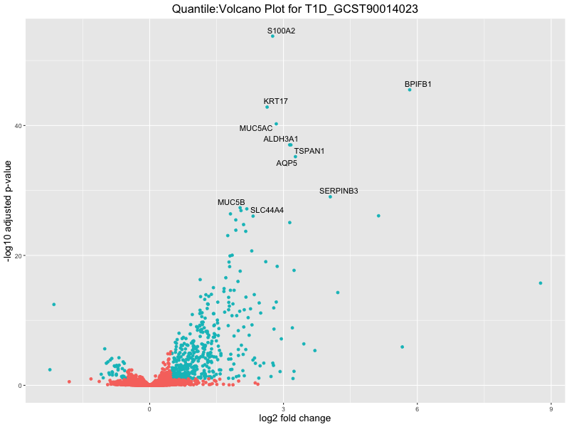
  volcano_plot <- ggplot(res_tableOE, aes(x = log2FoldChange, y = -log10(padj))) +
    geom_point(aes(colour = threshold_OE)) +
    geom_text_repel(aes(label = genelabels)) +
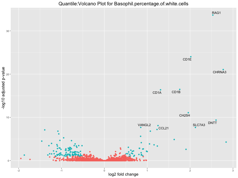
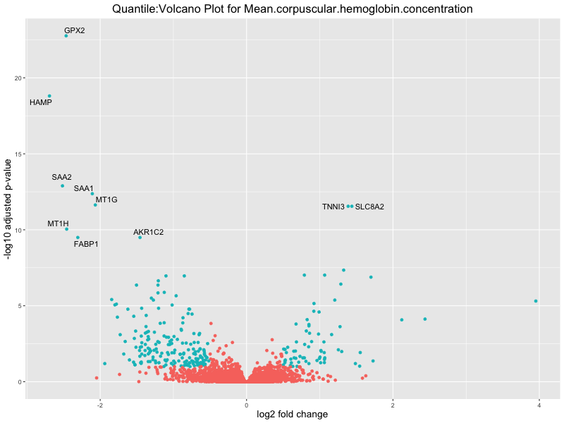
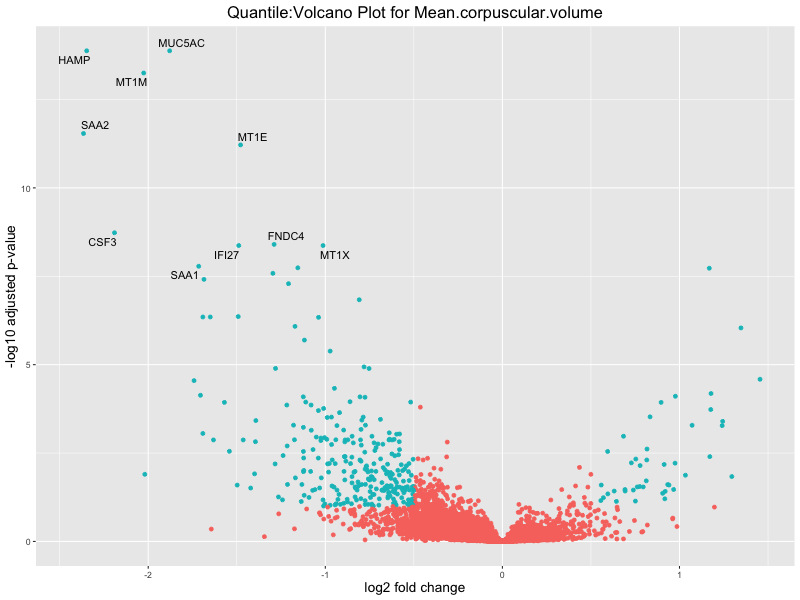
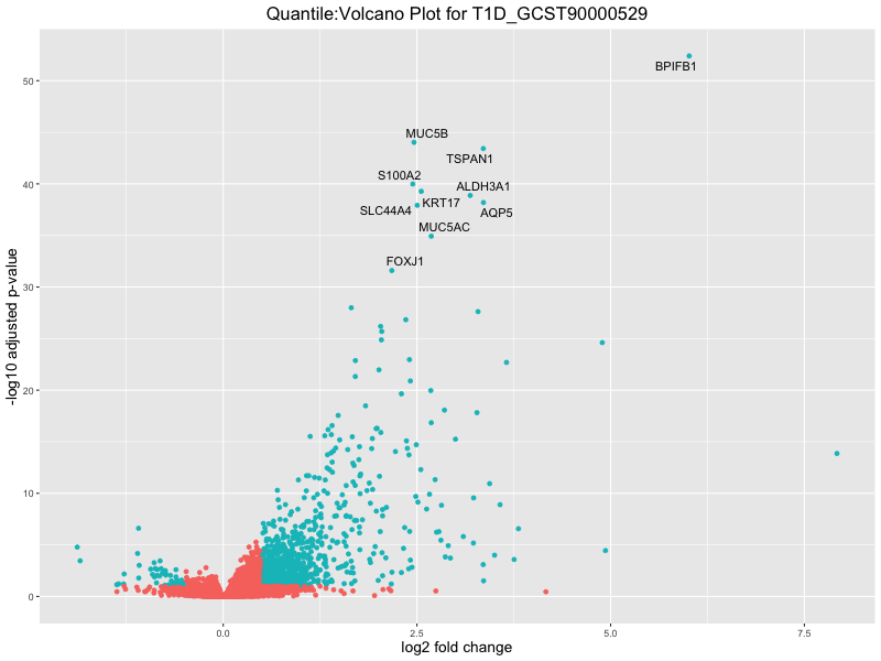
    ggtitle(paste("Quantile:Volcano Plot for", trait)) +
    xlab("log2 fold change") + 
    ylab("-log10 adjusted p-value") +
    theme(legend.position = "none",
          plot.title = element_text(size = rel(1.5), hjust = 0.5),
          axis.title = element_text(size = rel(1.25)))
  
  # Save the volcano plot
  png(paste0("volcano_plot_quantile_", trait, ".png"), width = 800, height = 600)
  print(volcano_plot)
  dev.off()
}

Model 2: expression ~ PRS + sex + expression PCs + 2 genotype PCs

Continuous PRS:

# Load the gene expression data
gene_expr_file <- "data/gene_reads_2017-06-05_v8_whole_blood.gct"
raw_count_df <- fread(gene_expr_file, header = TRUE, sep = "\t", drop = "id")

# load protein_coding list
protein_coding <- fread("data/protein-coding_gene.txt", 
                        sep = "\t")
protein_coding <- protein_coding[, c("symbol", "ensembl_gene_id")]

# keep only protein-coding genes
raw_count_df <- raw_count_df[raw_count_df$Description %in% protein_coding$symbol, ]

id <- raw_count_df$Name
raw_count <- raw_count_df[, -c(1:2)]

# modify GTEx sample names matching names used in PRS data
colnames(raw_count) <- sub("^(GTEX-[^-.]+).*", "\\1", colnames(raw_count))

matching_samples <- intersect(rownames(metadata), colnames(raw_count))
final_count <- raw_count[ , ..matching_samples]

# prefilter: keep only rows that have a count of at least 10
keep_genes <- rowSums(final_count >= 10) > 0
final_count <- final_count[keep_genes, ]
id <- id[keep_genes]
dim(final_count)

[1] 16893   670

# obtain genotype PCs
geno_pc <- read.table("data/pca.eigenvec")
names(geno_pc) = c("FID","IID",paste0("geno_PC", c(1:(ncol(geno_pc)-2))))

eigenval <- scan("data/pca.eigenval")
pve <- data.frame(PC = 1:20, pve = eigenval/sum(eigenval)*100)

ggplot(geno_pc) + geom_point(aes(x = geno_PC1, y = geno_PC2)) + 
  labs(x = paste0("PC1 (", signif(pve$pve[1], 3), "%)"), 
       y = paste0("PC2 (", signif(pve$pve[2], 3), "%)")) + theme_classic()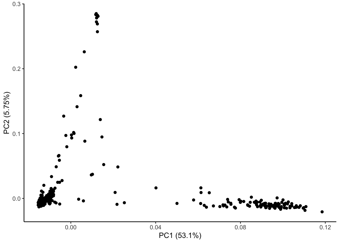

Version	Author	Date
51ffd48	ElisaChen	2025-05-20

ggplot(geno_pc) + geom_point(aes(x = geno_PC1, y = geno_PC3)) + 
    labs(x = paste0("PC1 (", signif(pve$pve[1], 3), "%)"), 
         y = paste0("PC3 (", signif(pve$pve[3], 3), "%)")) + theme_classic()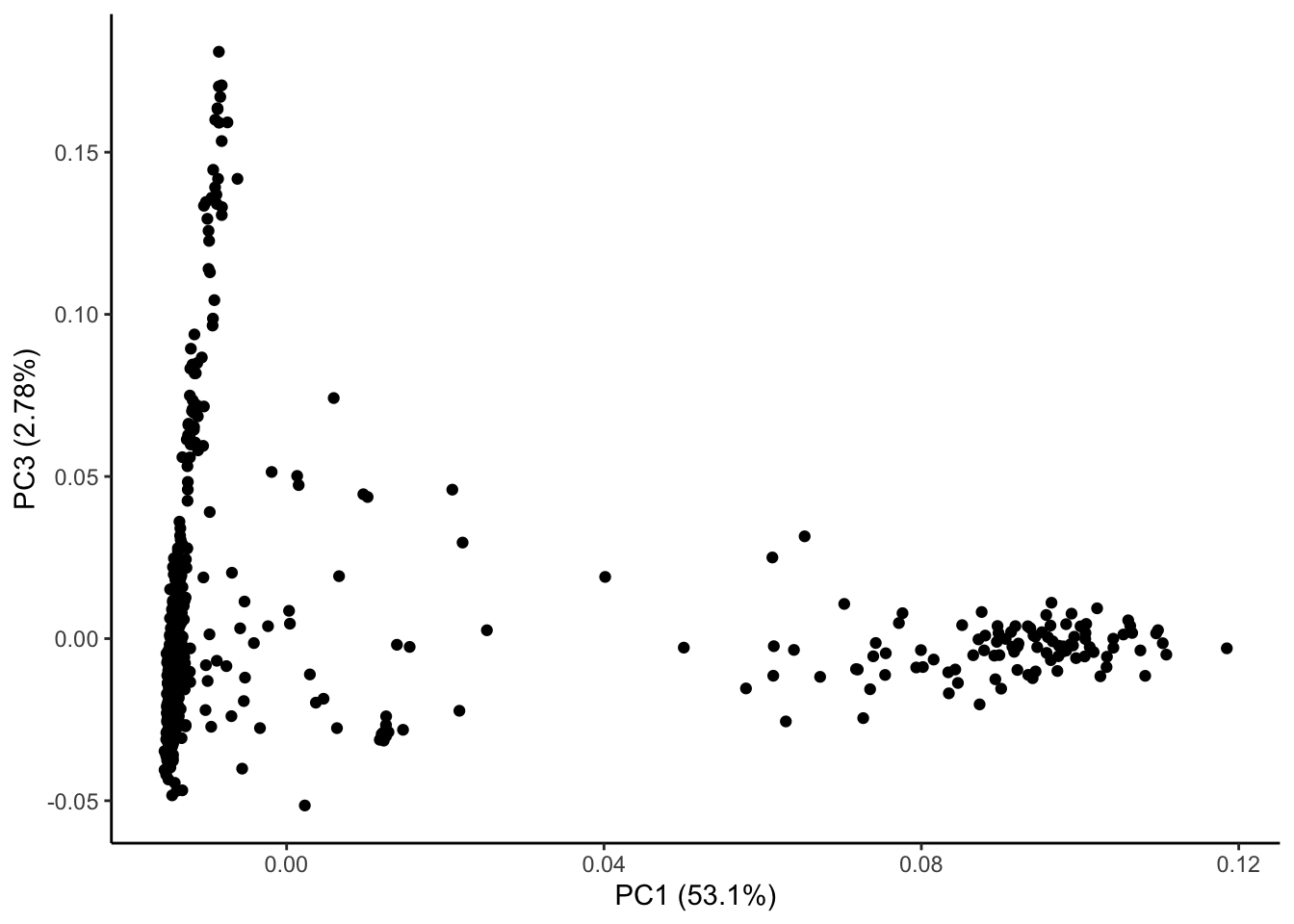

Version	Author	Date
51ffd48	ElisaChen	2025-05-20

ggplot(pve, aes(PC, pve)) + geom_point() + geom_line() +
  labs(x = "Genotype PC", y = "Percentage variance explained") + theme_classic()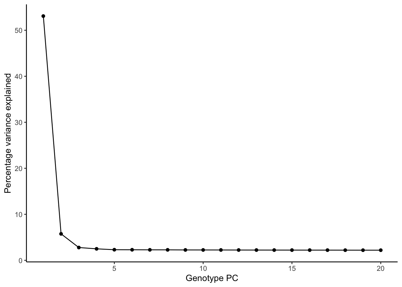

Version	Author	Date
51ffd48	ElisaChen	2025-05-20

metadata <- cbind(metadata, geno_pc[,3:ncol(geno_pc)])

# Loop through each trait and run DESeq2
for (trait in colnames(traits)) {
  
  # Standardize PRS for the current trait
  prs_trait <- traits[,trait]
  prs_trait <- scale(prs_trait) # Standardize PRS to mean = 0, sd = 1
    
  # Add the standardized PRS to the metadata for continuous trait
  metadata[,trait] <- prs_trait
  
  # Create the DESeqDataSet for the current trait
  dds <- DESeqDataSetFromMatrix(
    countData = as.matrix(final_count),  # Raw counts
    colData = metadata[, c(1:6, 44:45, which(colnames(metadata) == trait))],
    design = as.formula(paste("~ PC1 + PC2 + PC3 + PC4 + PC5 + sex + geno_PC1 + geno_PC2 +", trait))
  )
  rownames(dds) <- id
  
  # Run DESeq2 analysis
  dds <- DESeq(dds, parallel = TRUE, BPPARAM = MulticoreParam(4))
  
  # Get the results for the current trait
  res <- results(dds)
  
  # Save the results to a file
  write.csv(res, paste0("differential_expression_", trait, "_results_M2.csv"))
  
  # print a summary of the results
  print(paste("Results for trait:", trait))
  print(summary(res))
  
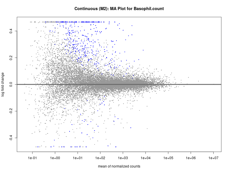
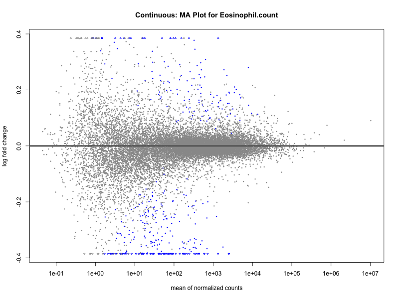
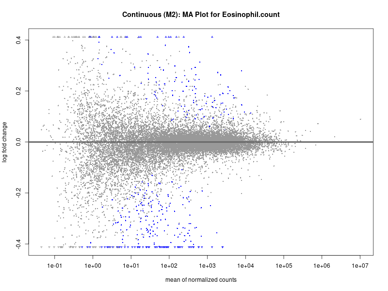
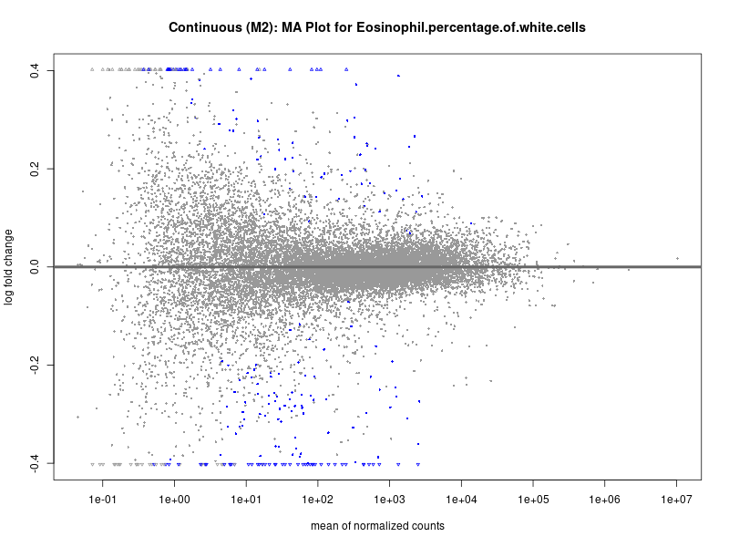
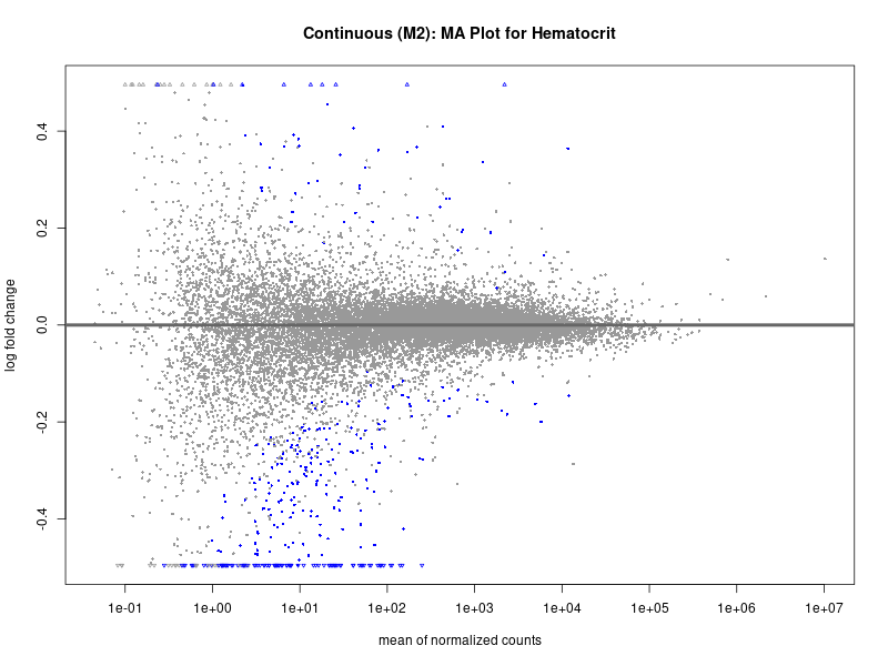
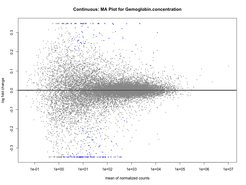
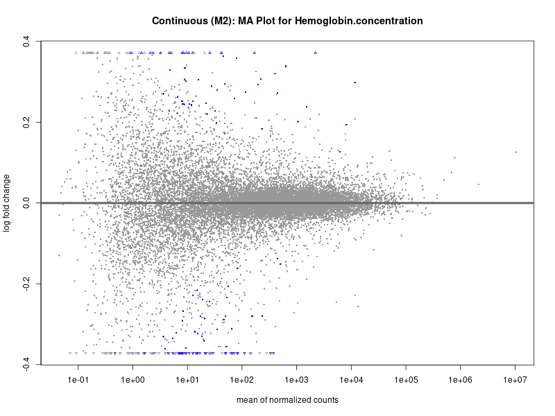
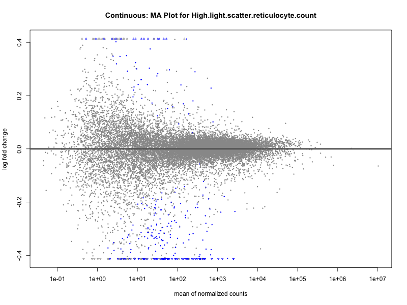
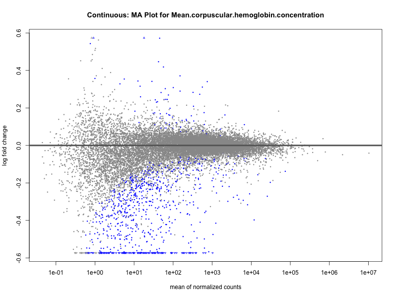
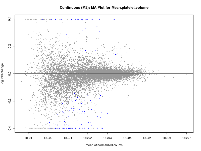
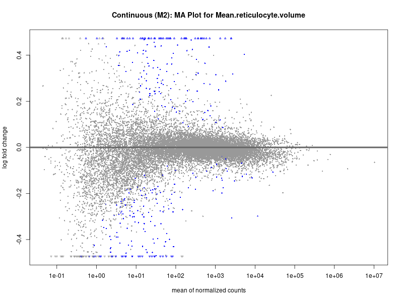
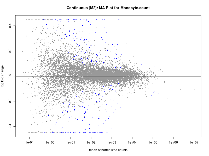
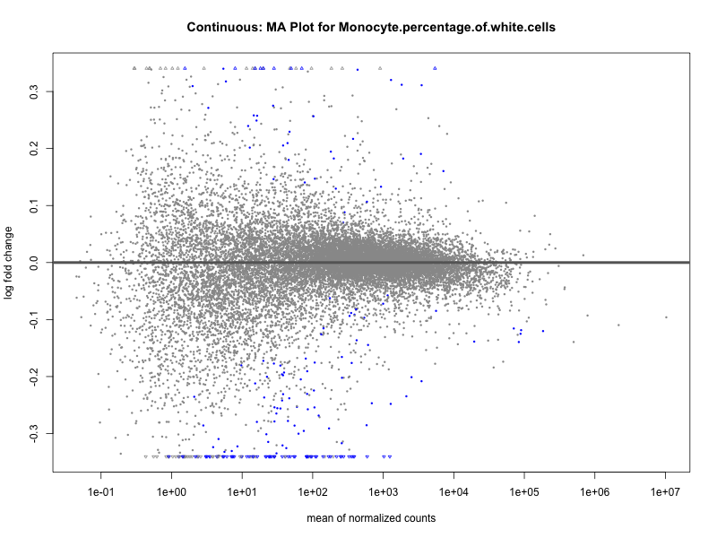
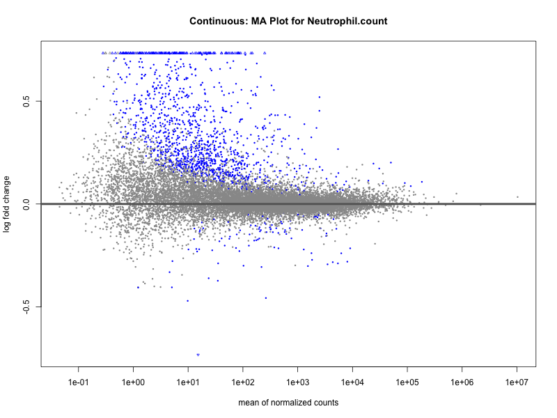
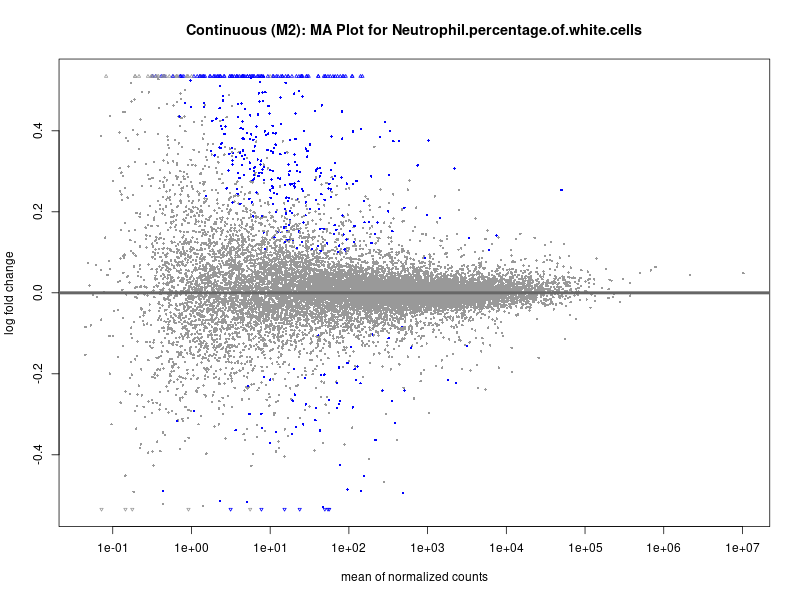
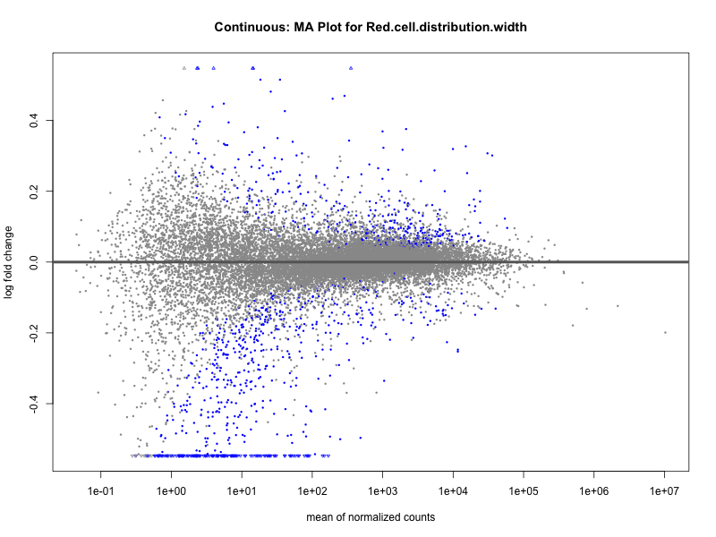
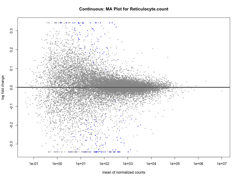
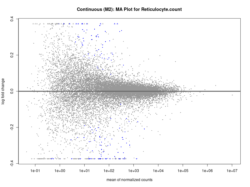
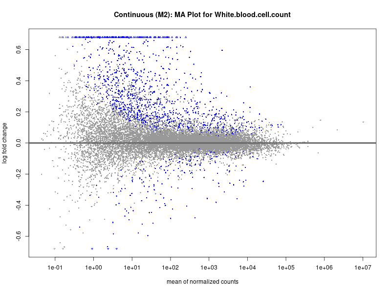
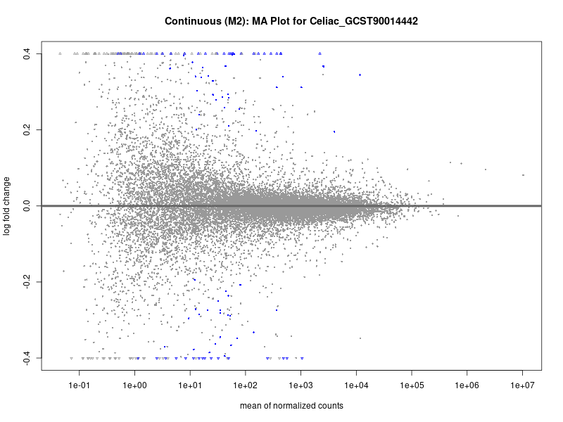
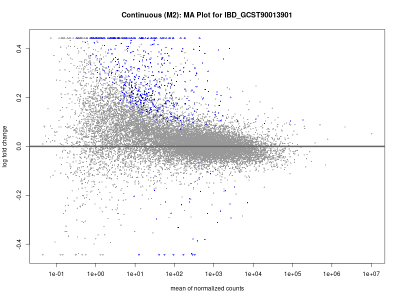
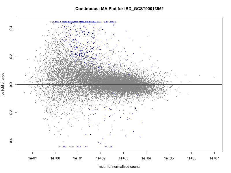
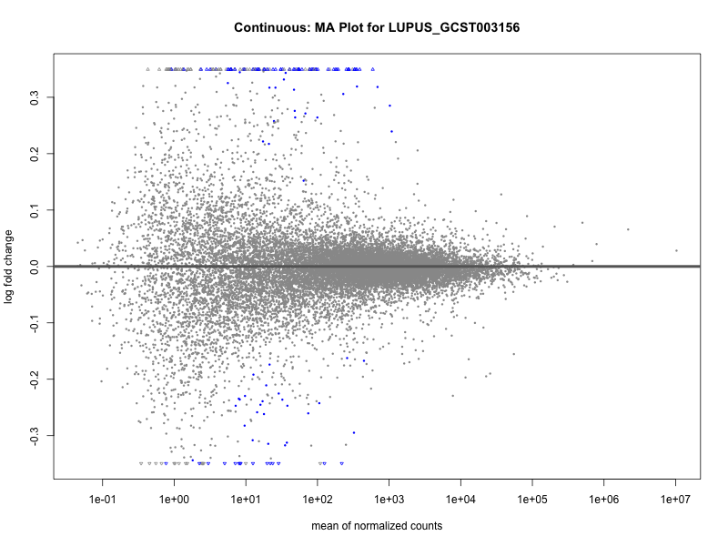
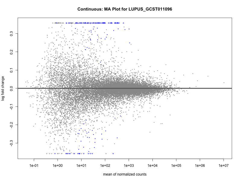
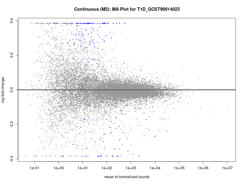
  # plot the MA-plot for the current trait
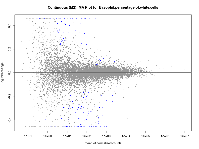
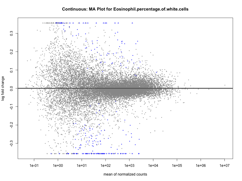
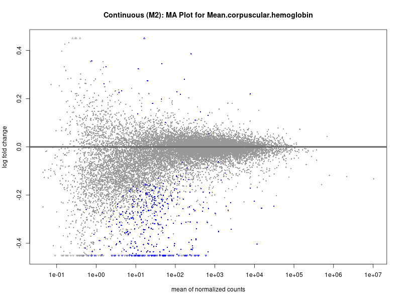
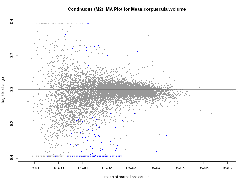
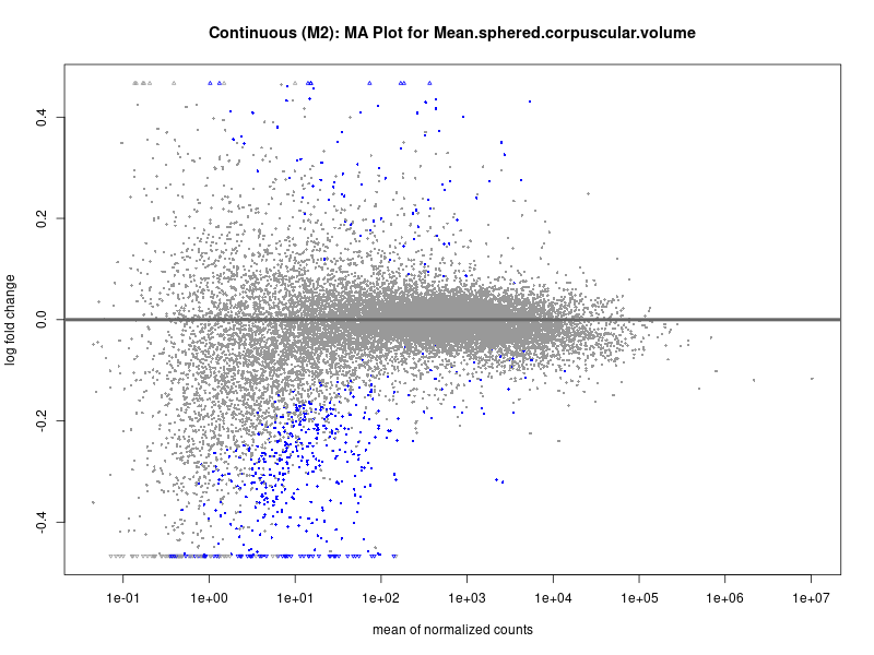
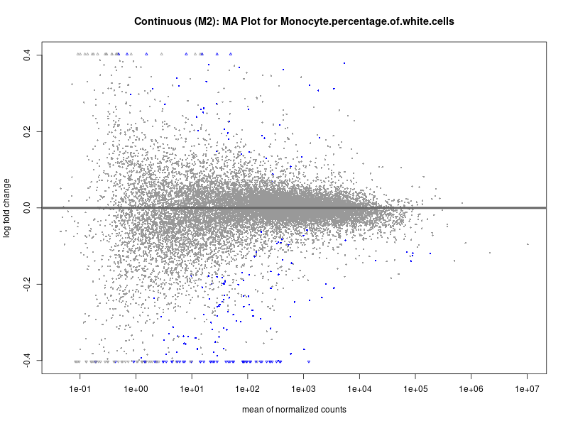
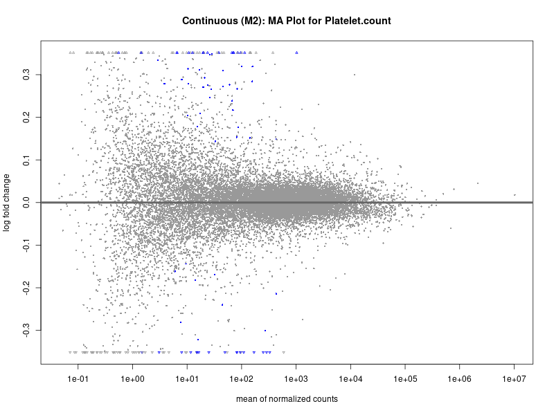
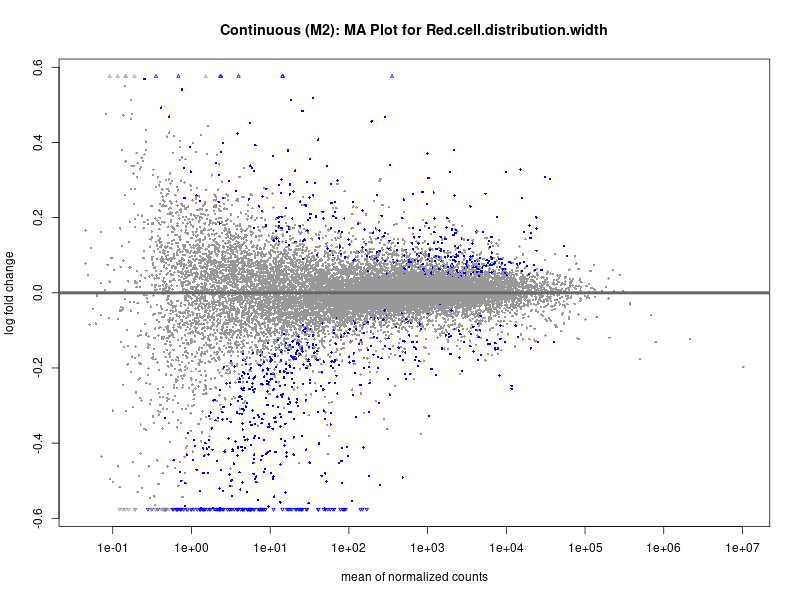
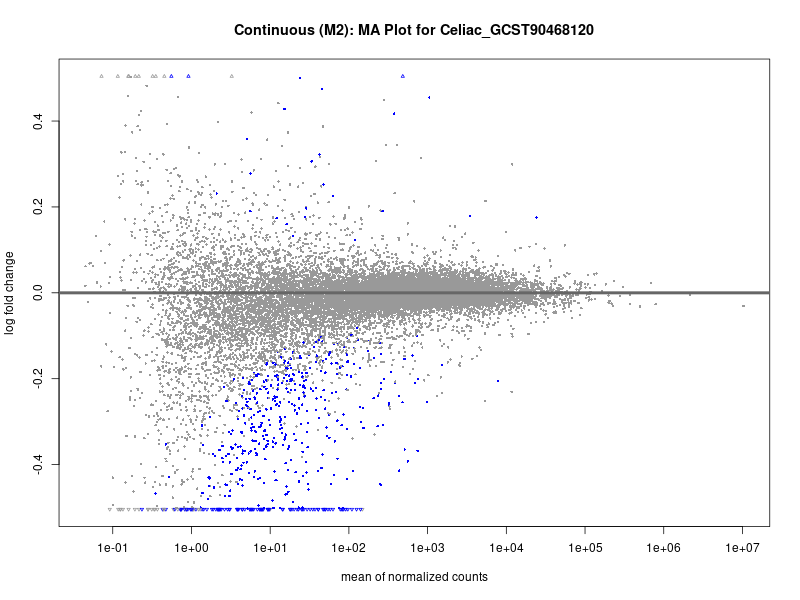
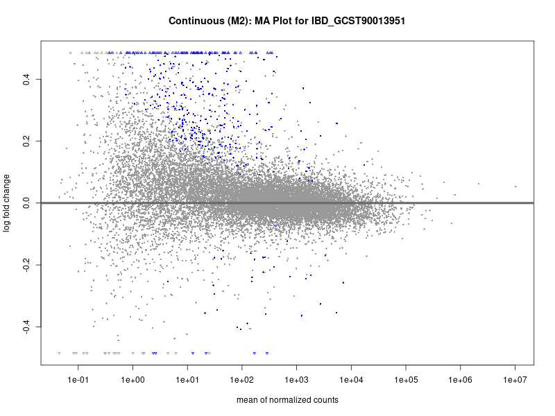
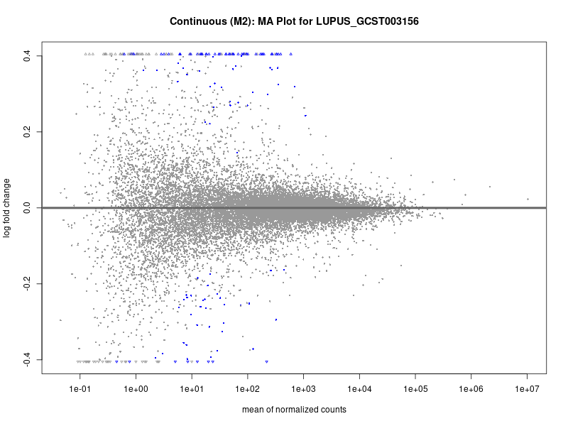
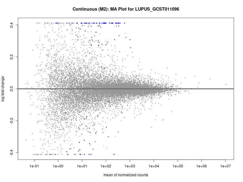
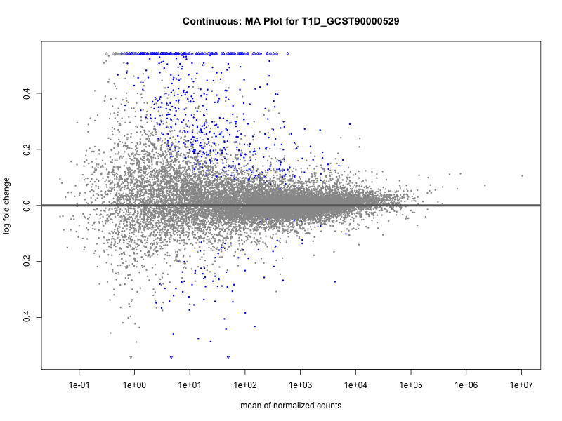
  png(paste0("ma_plot_", trait, "_M2.png"), width = 800, height = 600)
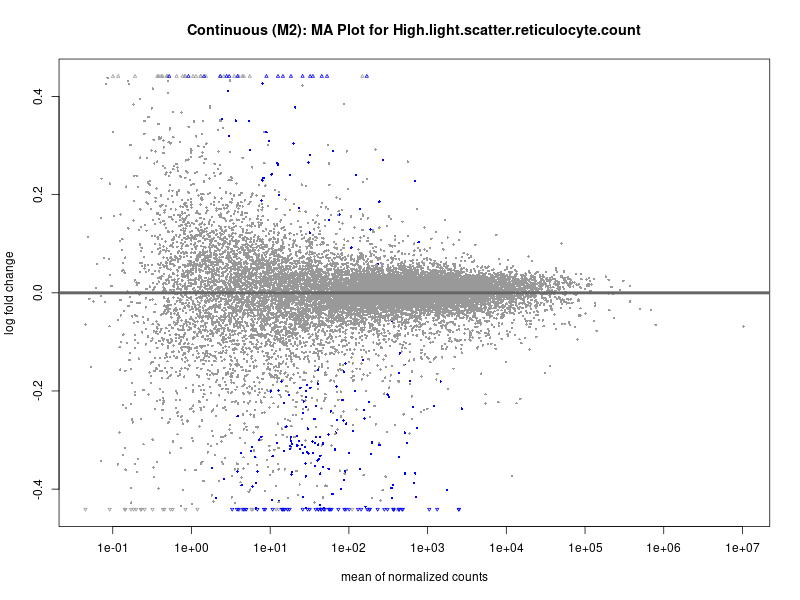
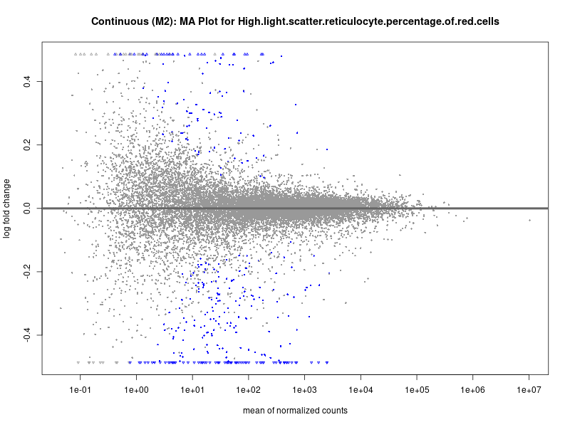
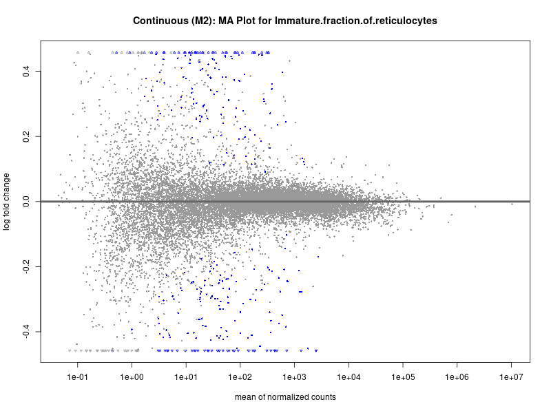
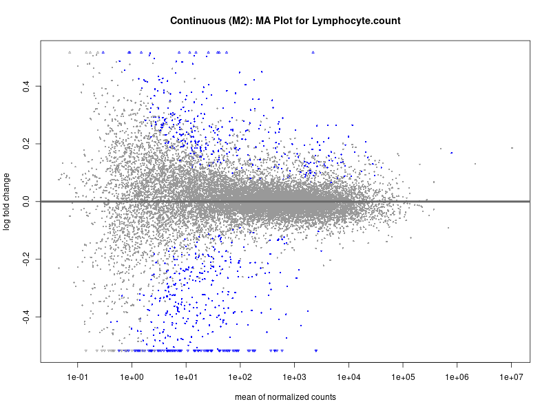
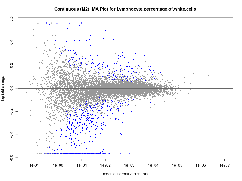
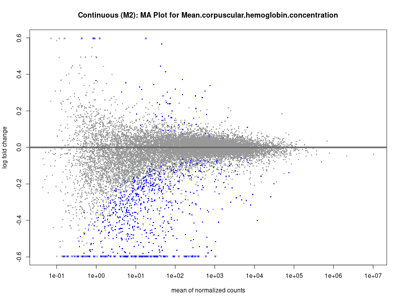
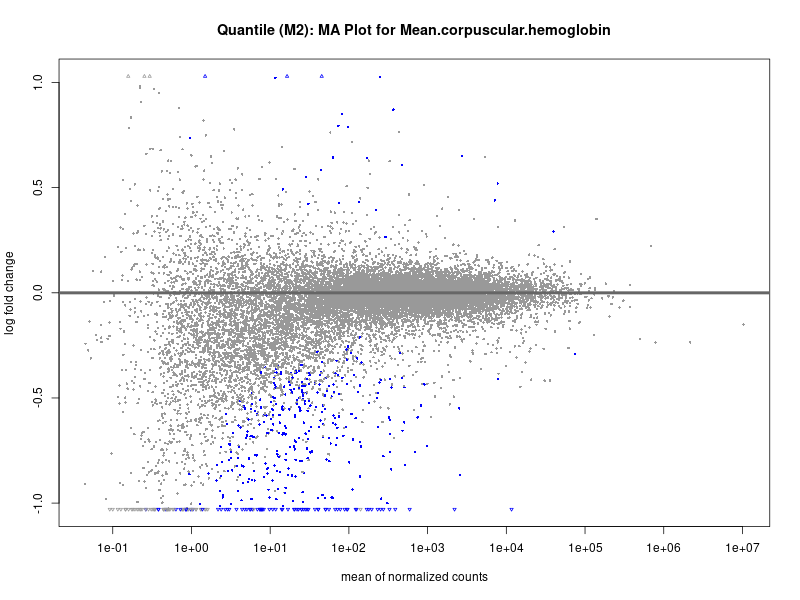
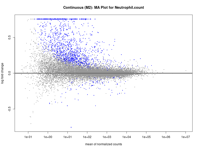
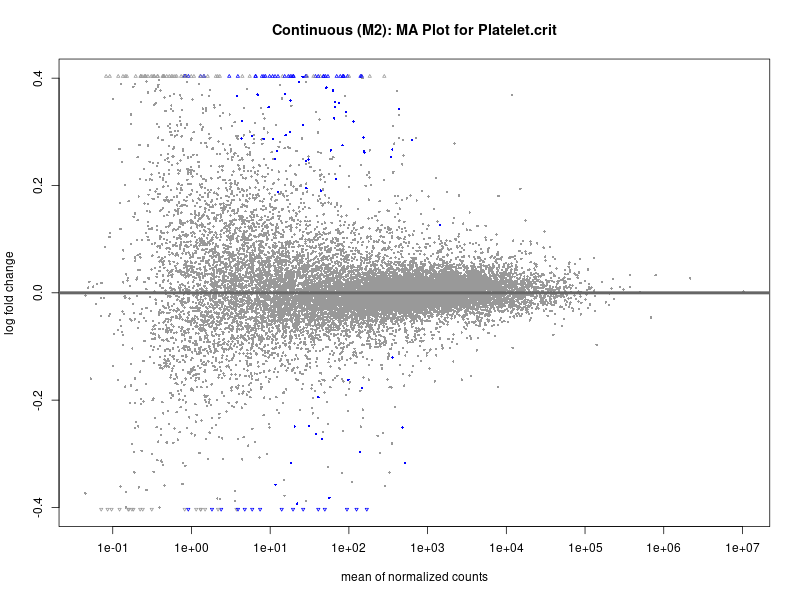
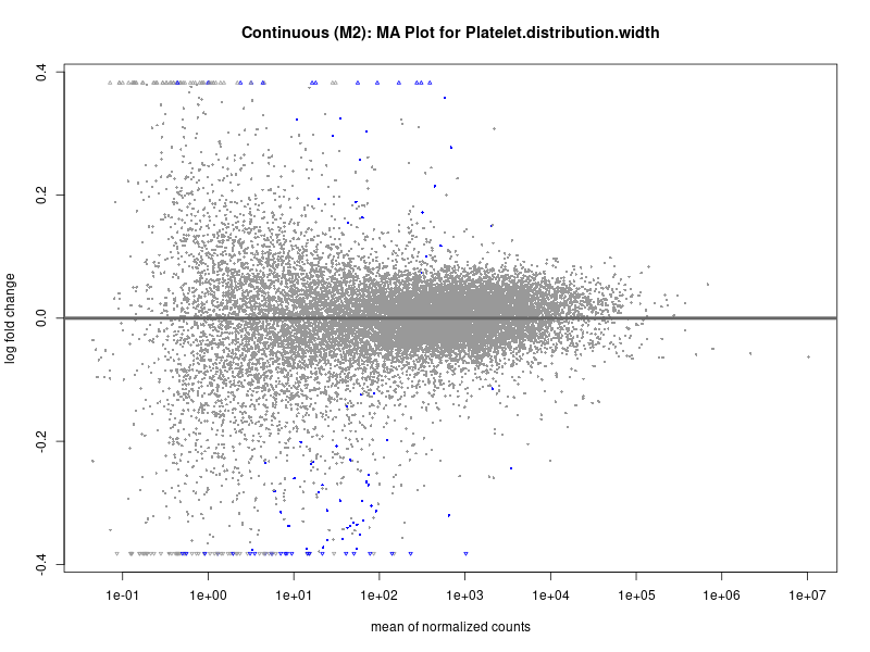
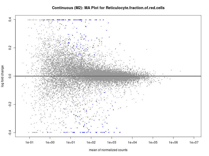
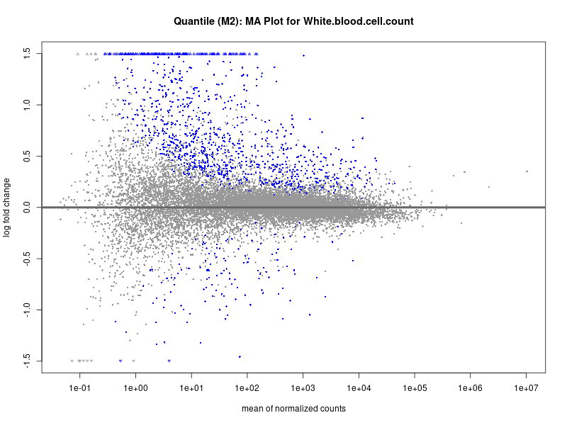
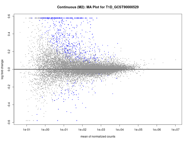
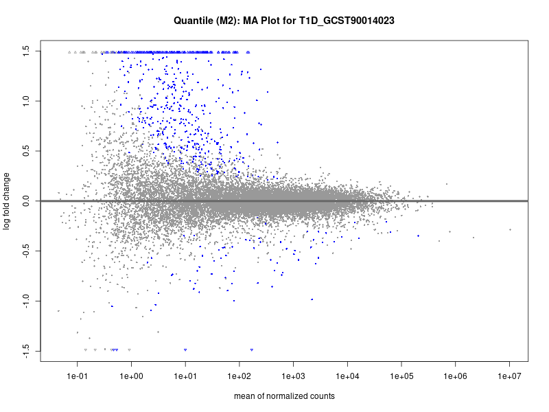
  plotMA(res, main = paste("Continuous (M2): MA Plot for", trait))
  dev.off()
  
  # volcano plot
  res_tableOE <- as.data.frame(res)
  res_tableOE$gene_name <- raw_count_df$Description[keep_genes]
  res_tableOE <- mutate(res_tableOE, threshold_OE = padj < 0.1)
  res_tableOE <- res_tableOE %>% arrange(padj) %>% mutate(genelabels = "")
  res_tableOE$genelabels[1:10] <- res_tableOE$gene_name[1:10]
  
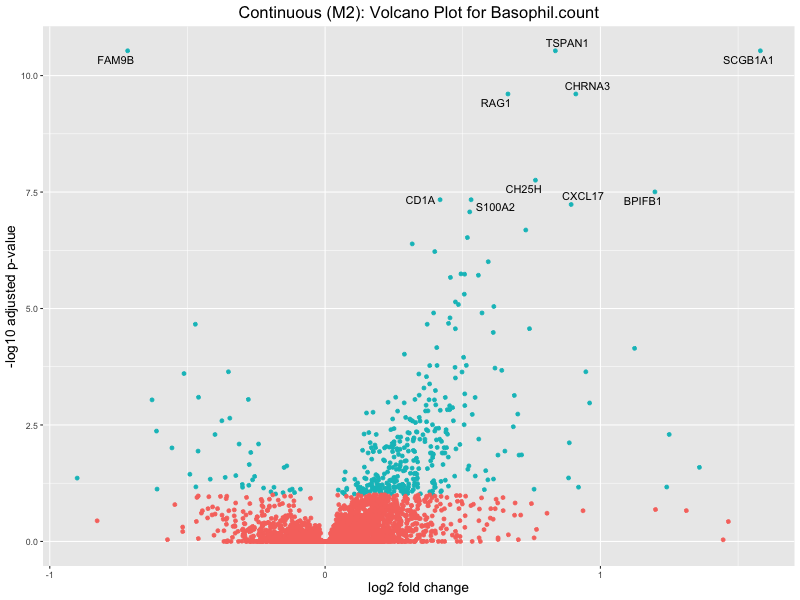
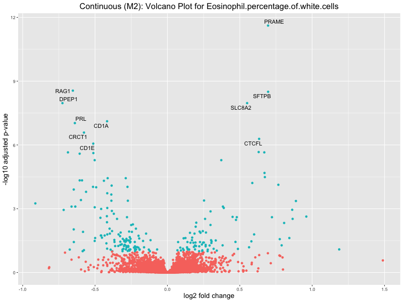
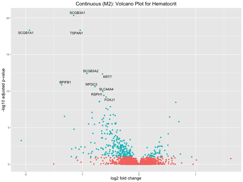
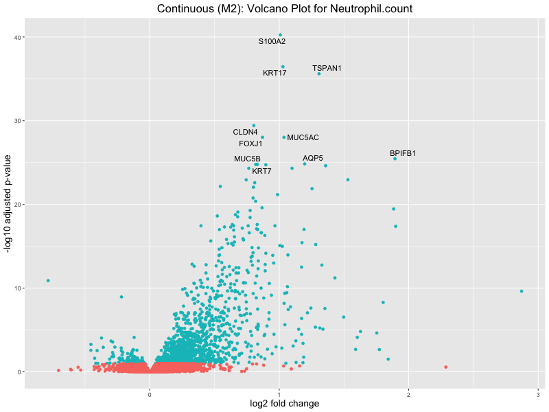
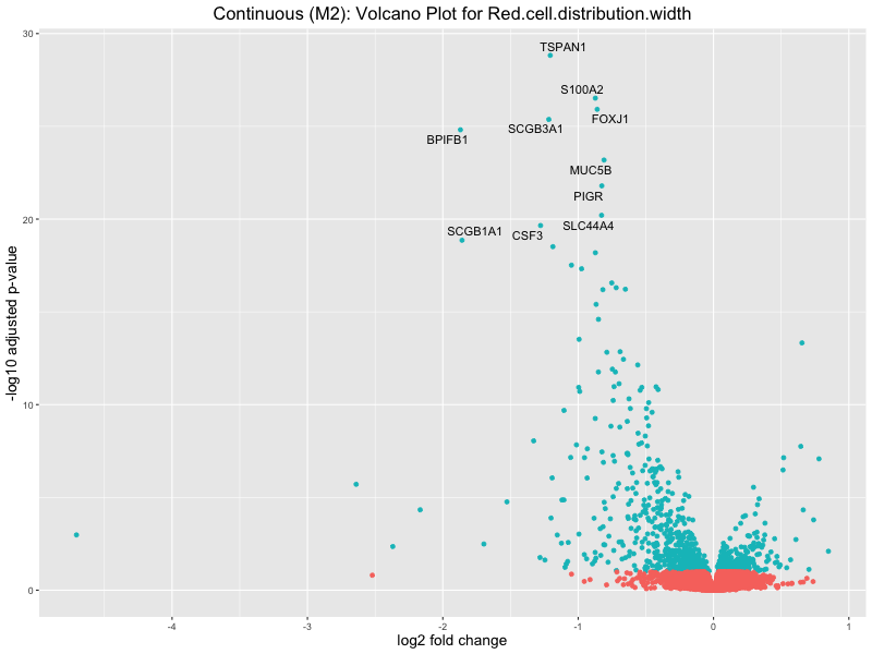
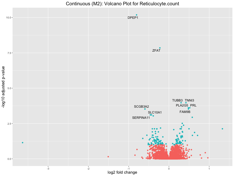
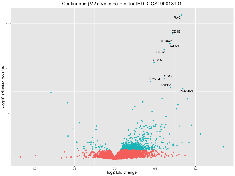
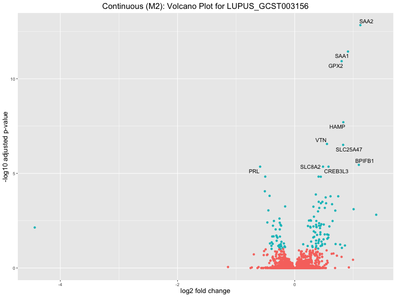
  volcano_plot <- ggplot(res_tableOE, aes(x = log2FoldChange, y = -log10(padj))) +
    geom_point(aes(colour = threshold_OE)) +
    geom_text_repel(aes(label = genelabels)) +
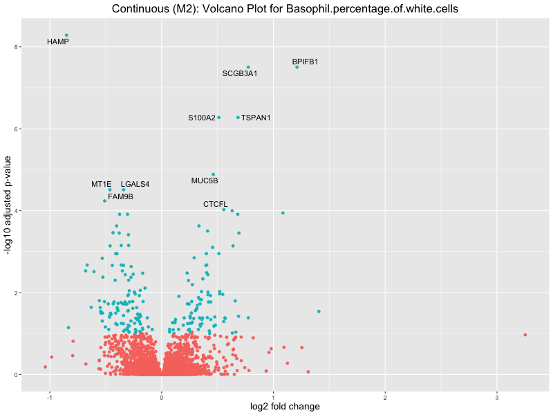
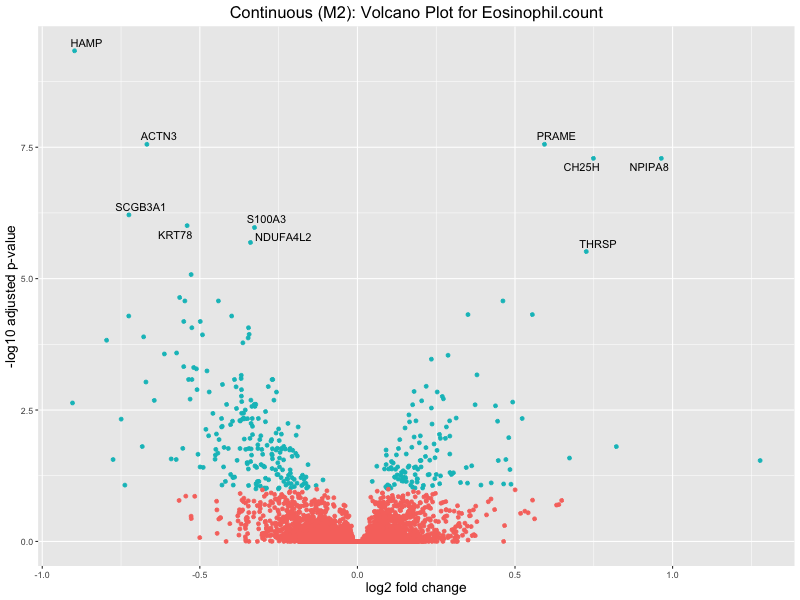
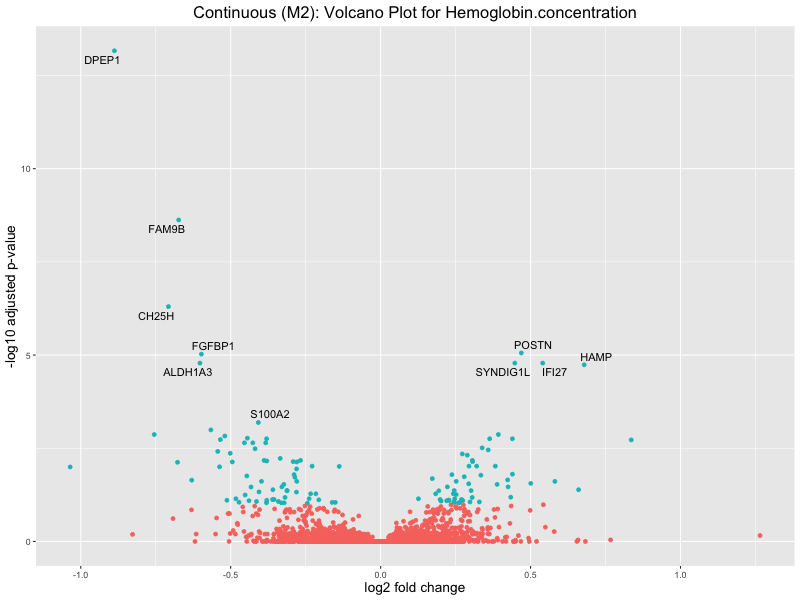
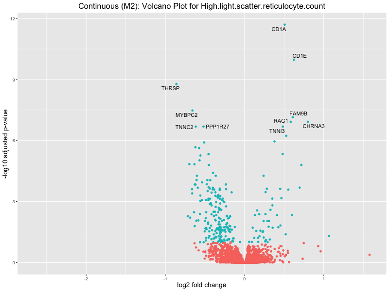
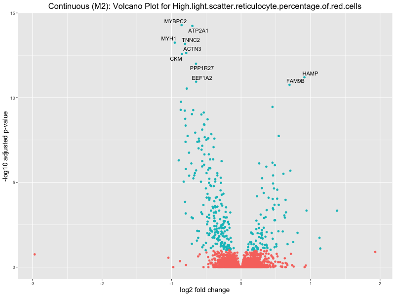
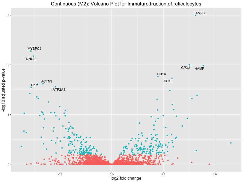
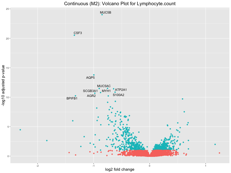
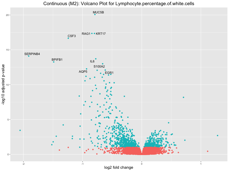
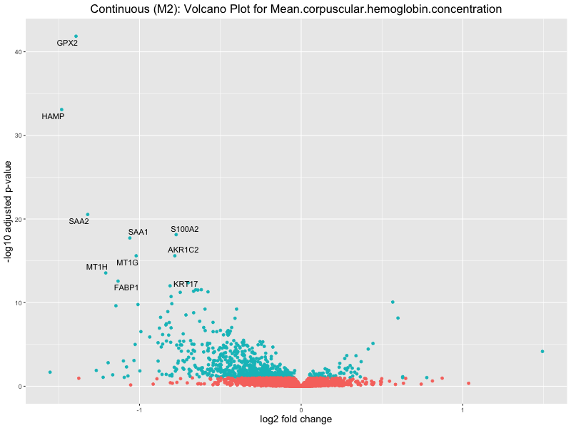
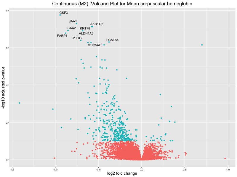
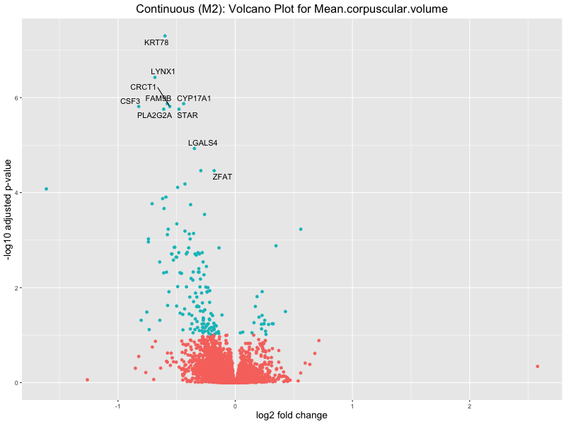
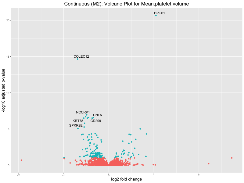
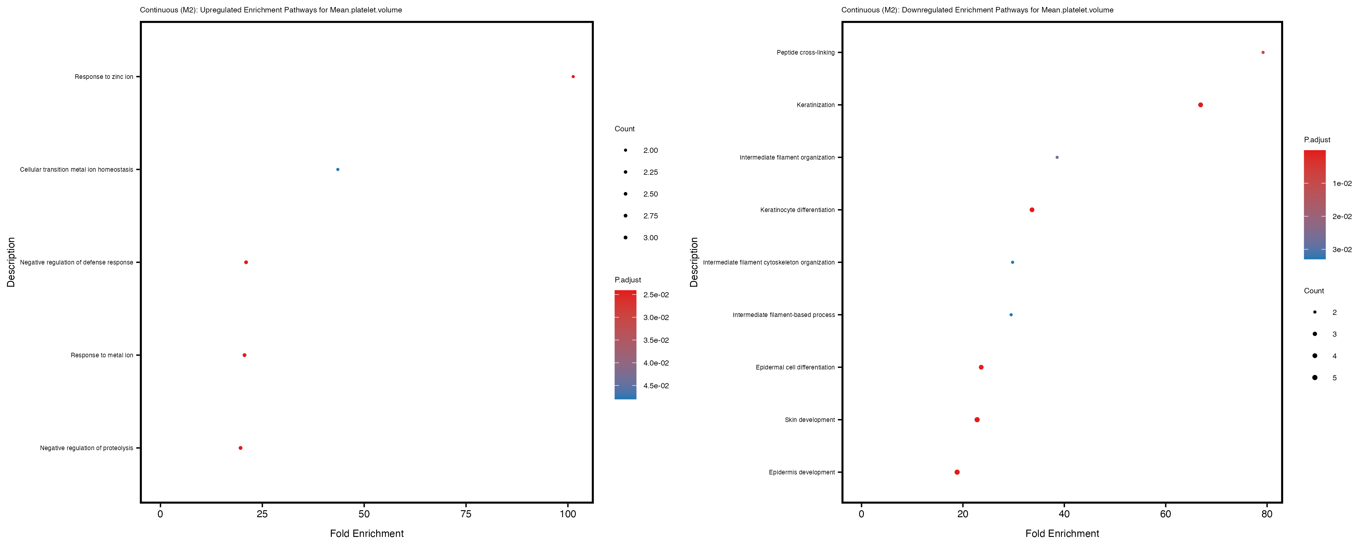
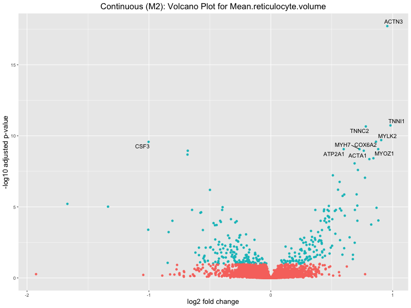
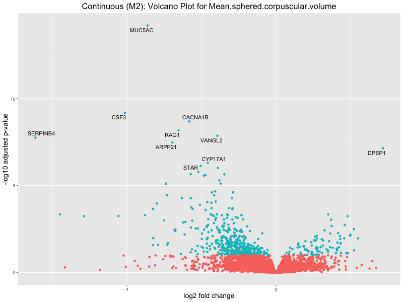
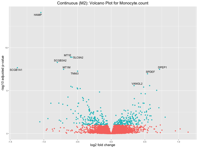
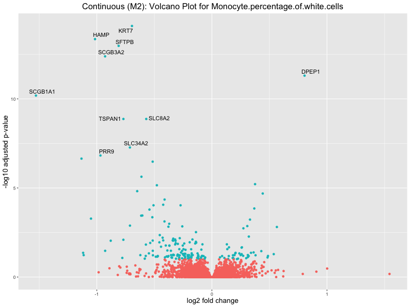
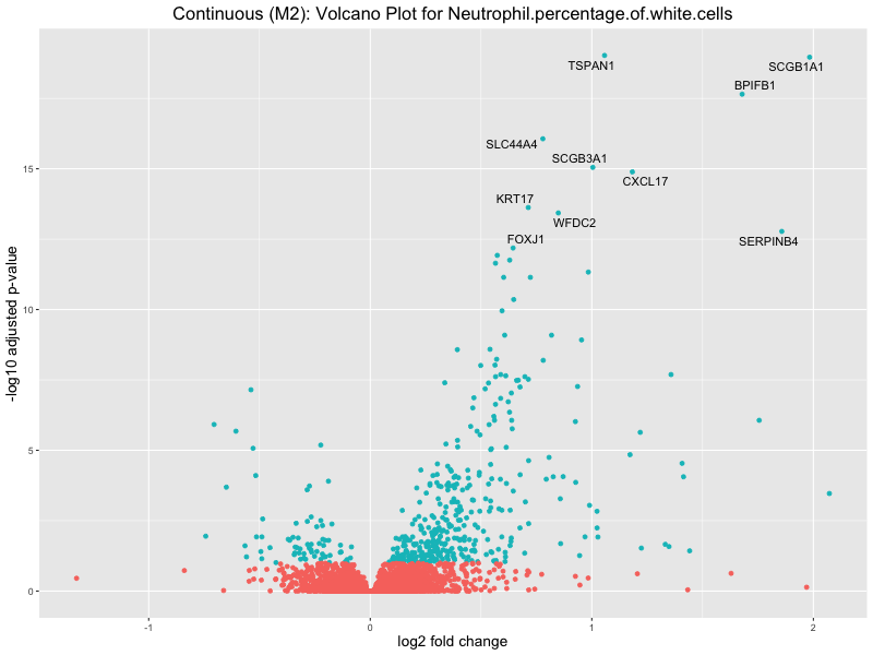
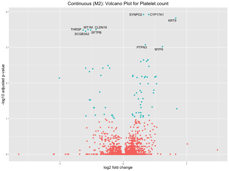
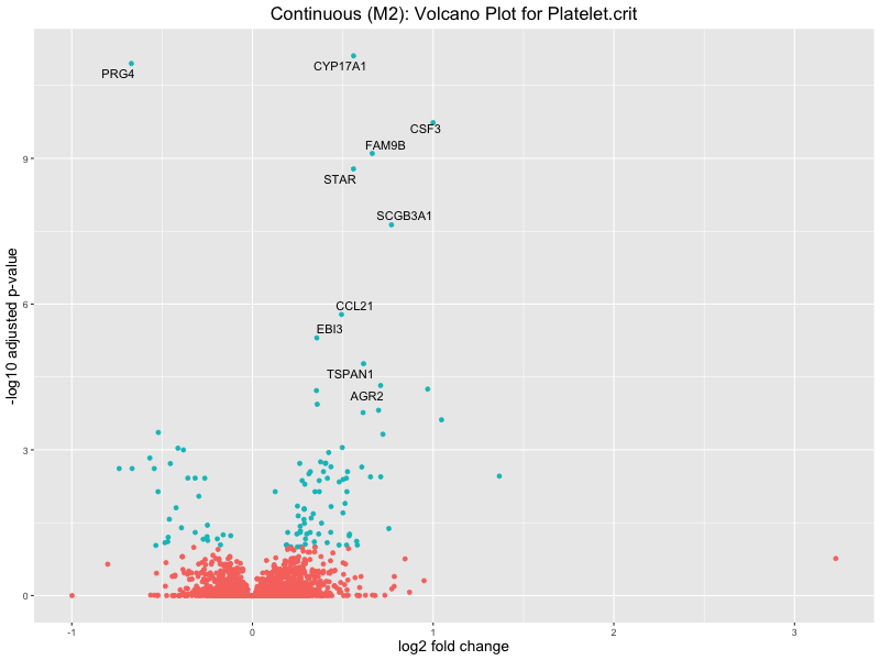
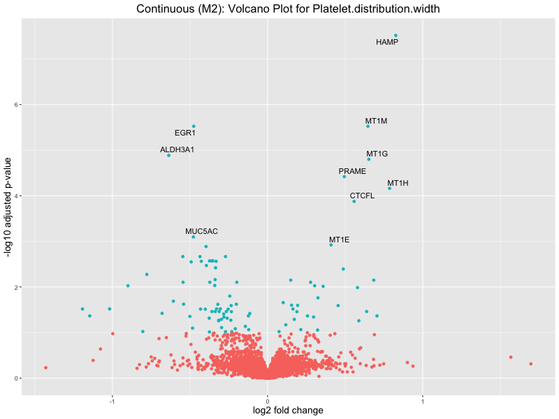
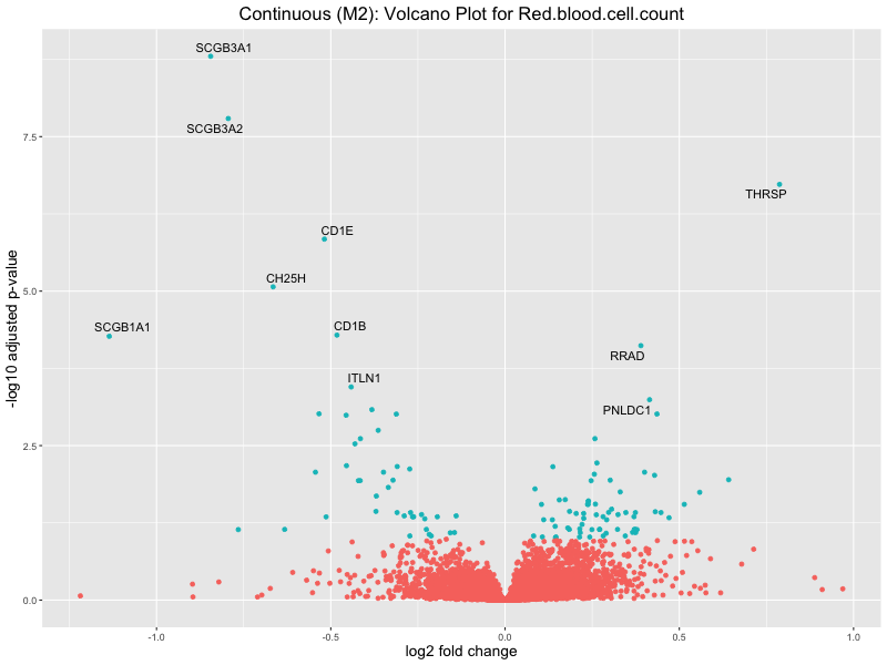
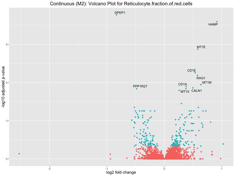
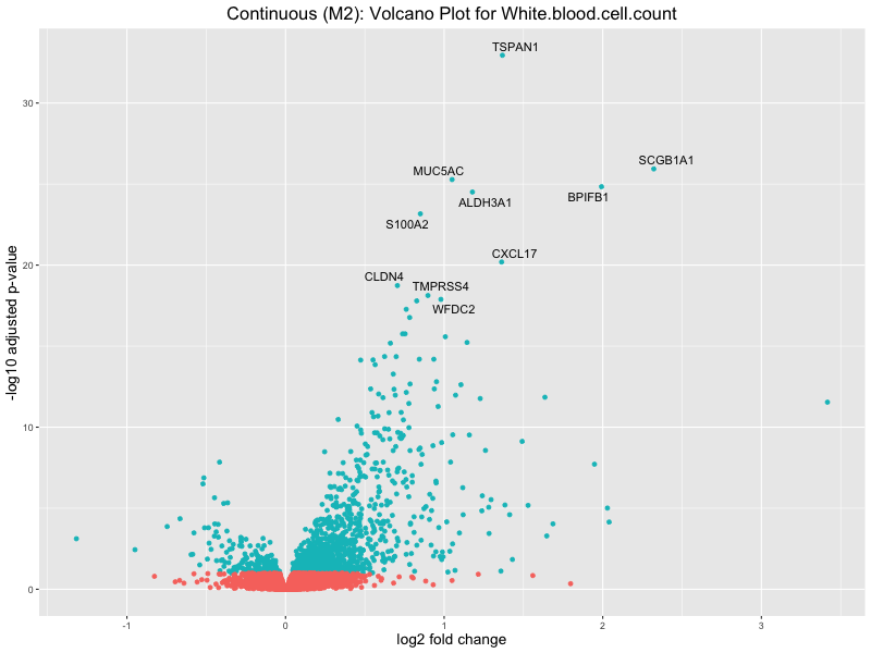
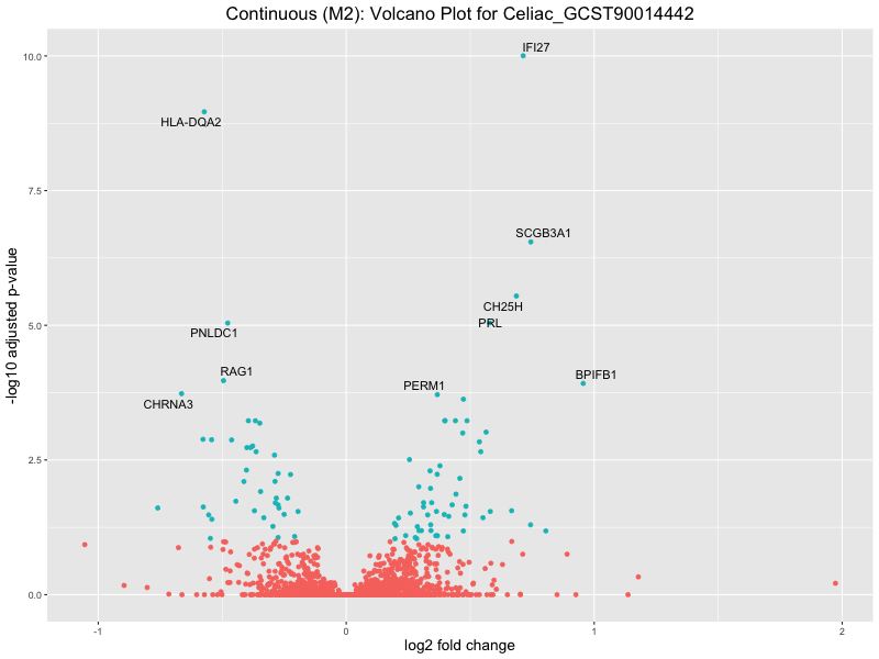
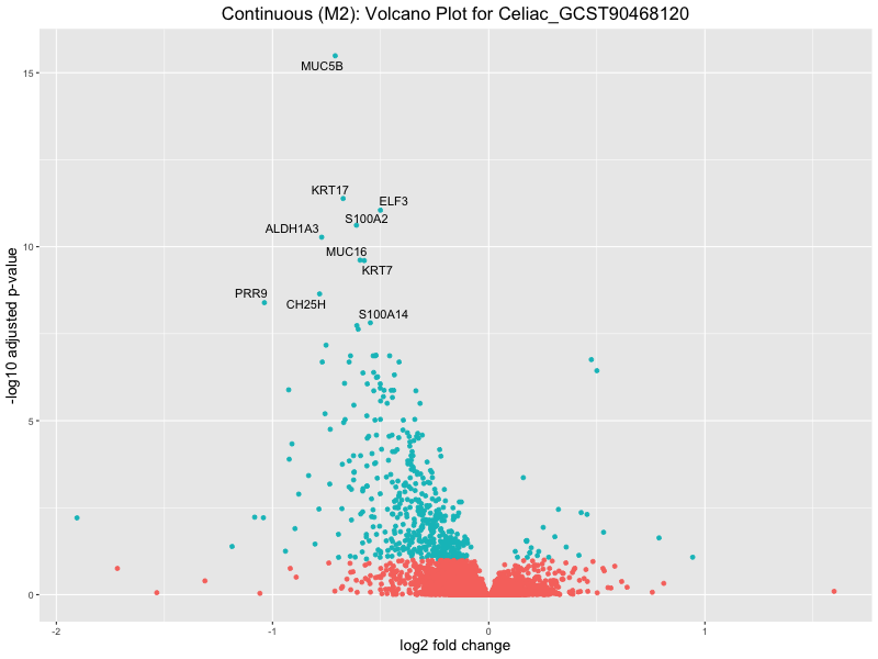
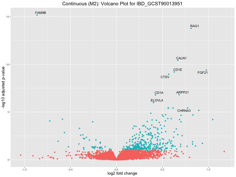
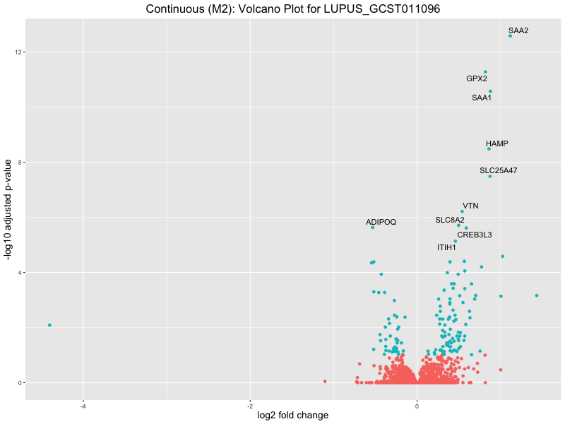
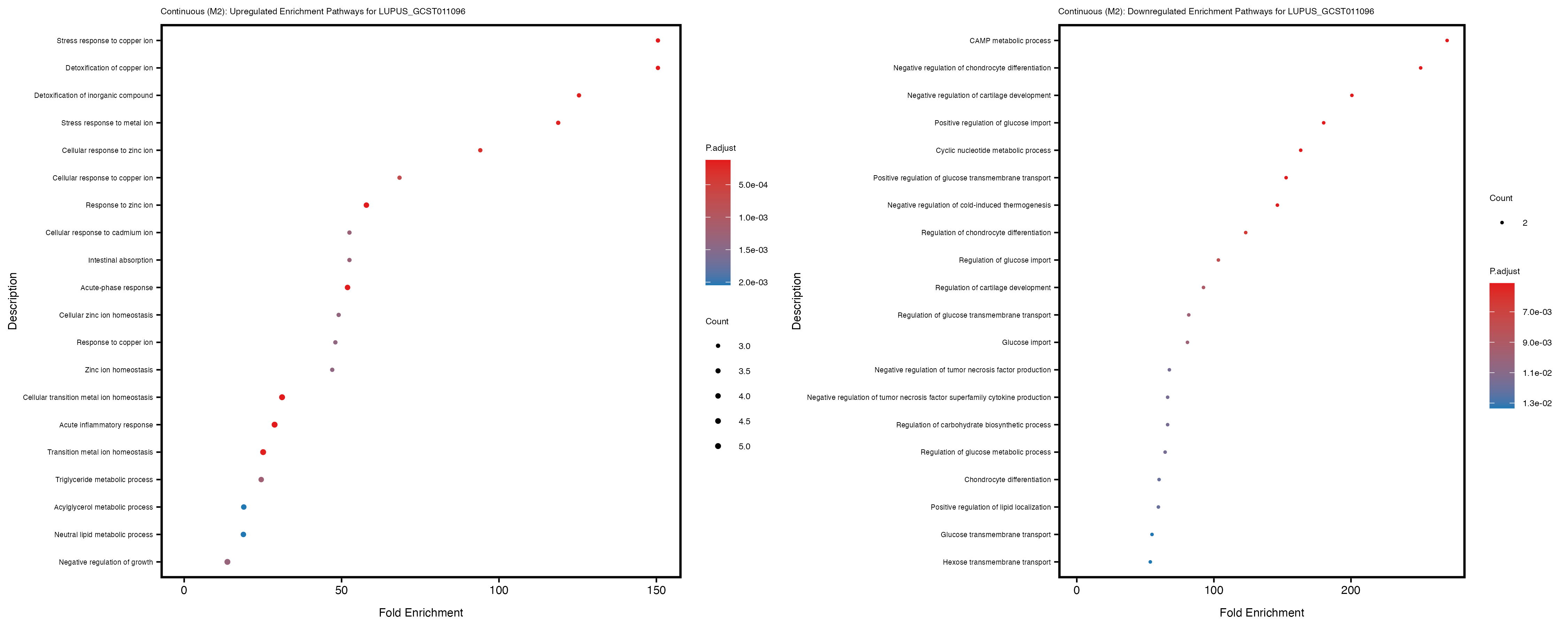
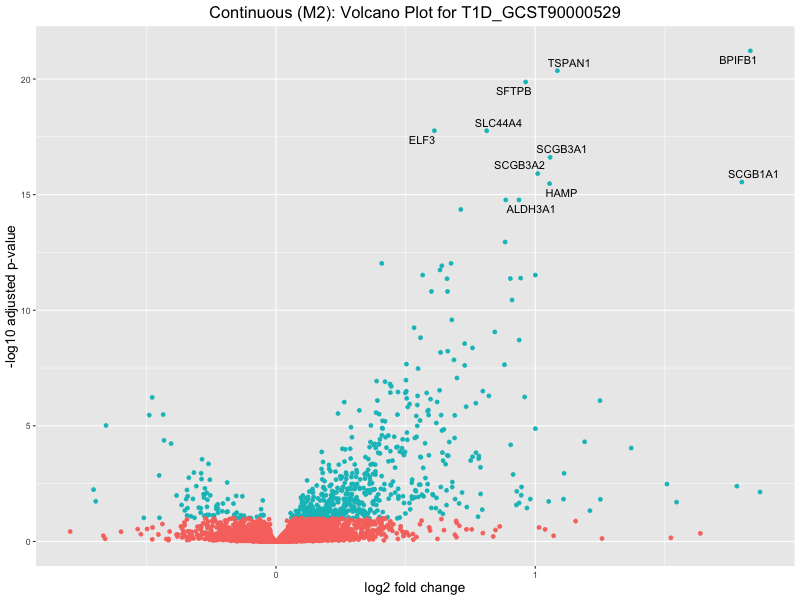
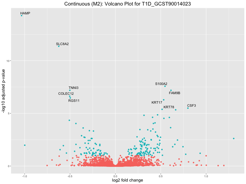
    ggtitle(paste("Continuous (M2): Volcano Plot for", trait)) +
    xlab("log2 fold change") + 
    ylab("-log10 adjusted p-value") +
    theme(legend.position = "none",
          plot.title = element_text(size = rel(1.5), hjust = 0.5),
          axis.title = element_text(size = rel(1.25)))
  
  # Save the volcano plot
  png(paste0("volcano_plot_", trait, "_M2.png"), width = 800, height = 600)
  print(volcano_plot)
  dev.off()
}

Quantile PRS:

metadata_file <- "analysis/metadata_quantile.txt"
metadata <- read.csv(metadata_file, header = T, sep = "\t", stringsAsFactors = T)
metadata$sex <- as.factor(metadata$sex)

traits <- metadata[, 7:43]

metadata <- cbind(metadata, geno_pc[,3:ncol(geno_pc)])

# Loop through each trait and run DESeq2
for (trait in colnames(traits)) {
  
  # Create the DESeqDataSet for the current trait
  dds <- DESeqDataSetFromMatrix(
    countData = as.matrix(final_count),  # Raw counts
    colData = metadata[, c(1:6, which(colnames(metadata) == trait))],
    design = as.formula(paste("~ PC1 + PC2 + PC3 + PC4 + PC5 + sex + geno_PC1 + geno_PC2 +", trait))
  )
  rownames(dds) <- id
  
  # Run DESeq2 analysis
  dds <- DESeq(dds, parallel = TRUE, BPPARAM = MulticoreParam(4))
  
  # Get the results for the current trait
  res <- results(dds)
  
  # Save the results to a file
  write.csv(res, paste0("differential_expression_", trait, "_quantile_results_M2.csv"))
  
  # print a summary of the results
  print(paste("Results for trait:", trait))
  print(summary(res))
  
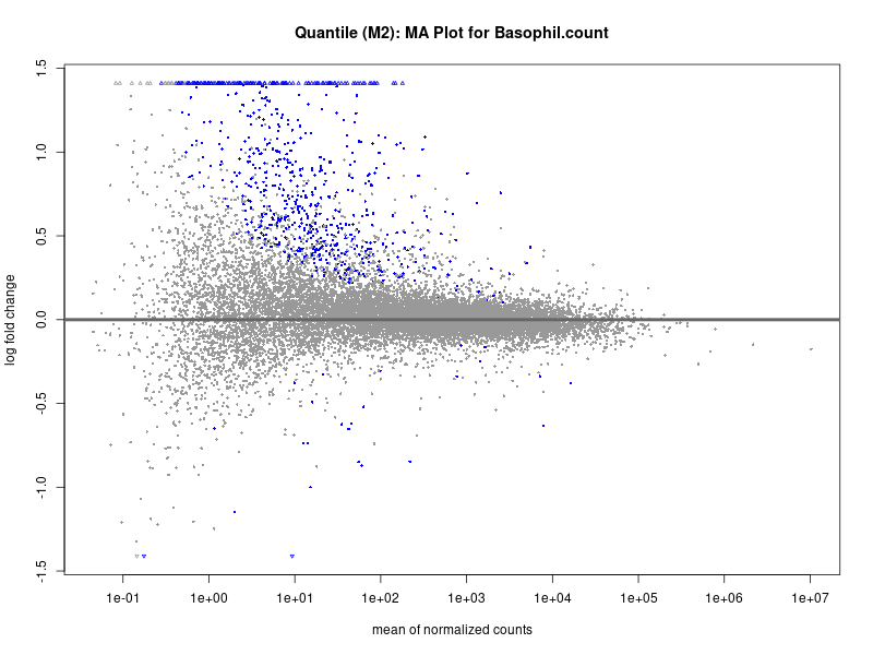
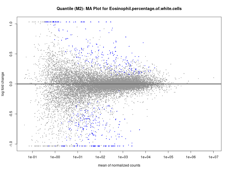
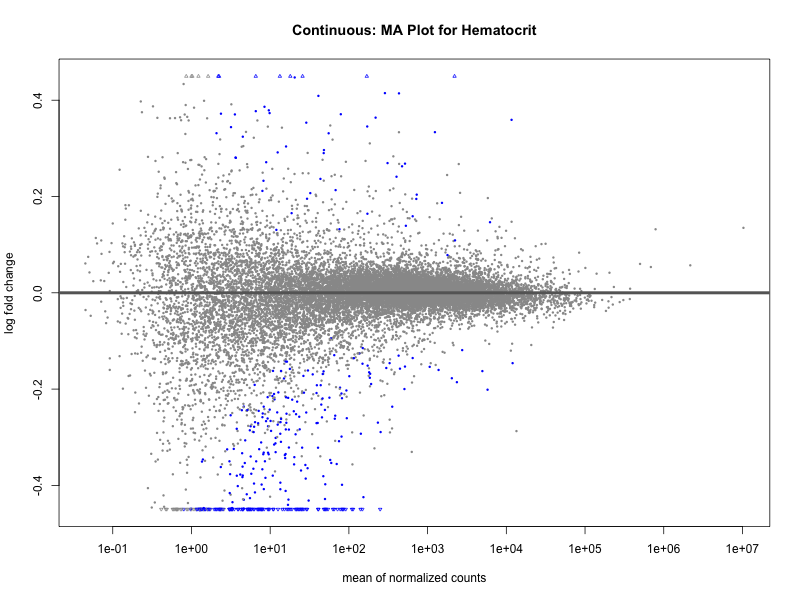
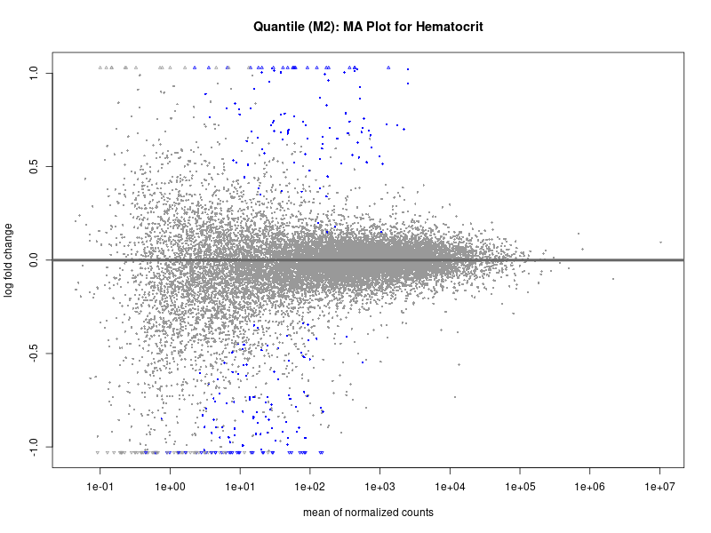
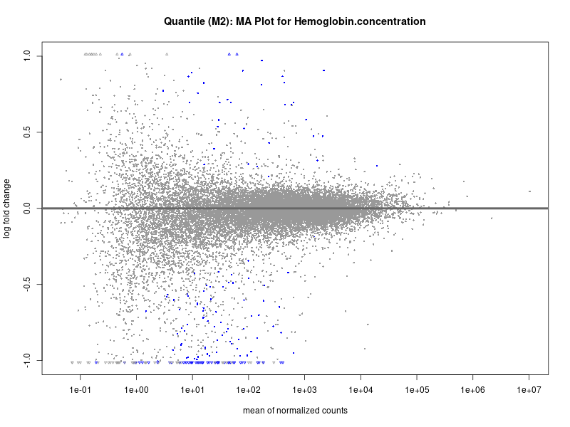
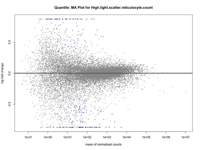
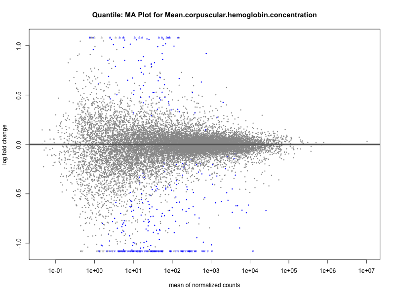
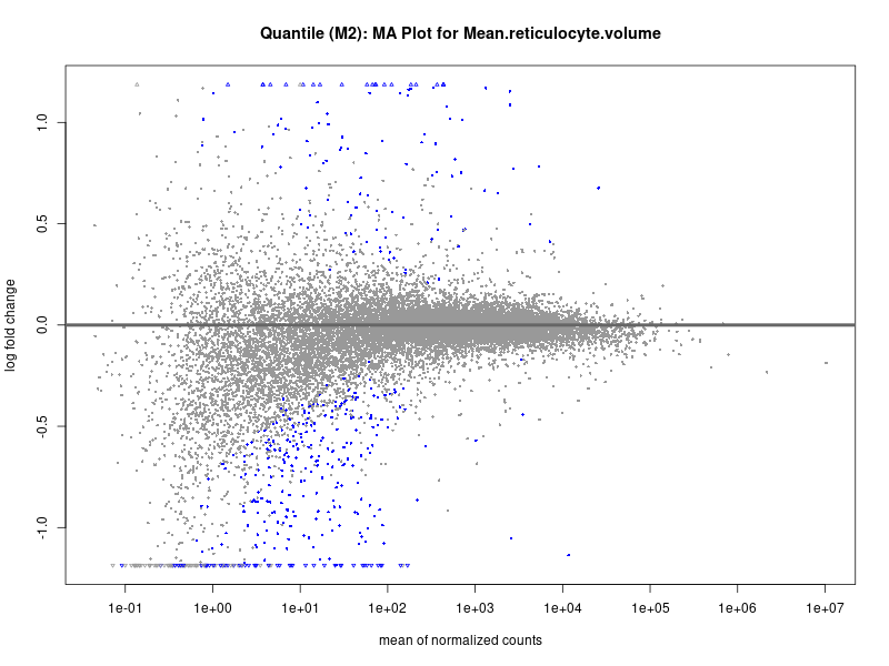
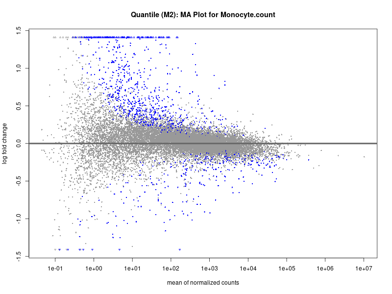
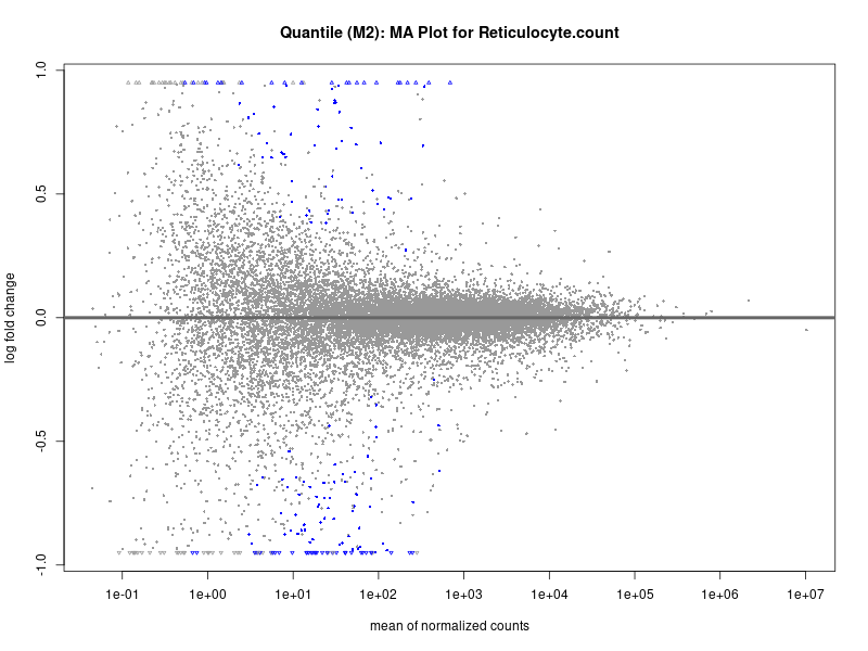
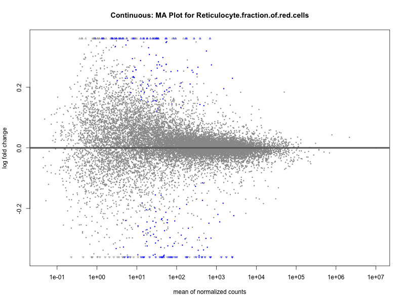
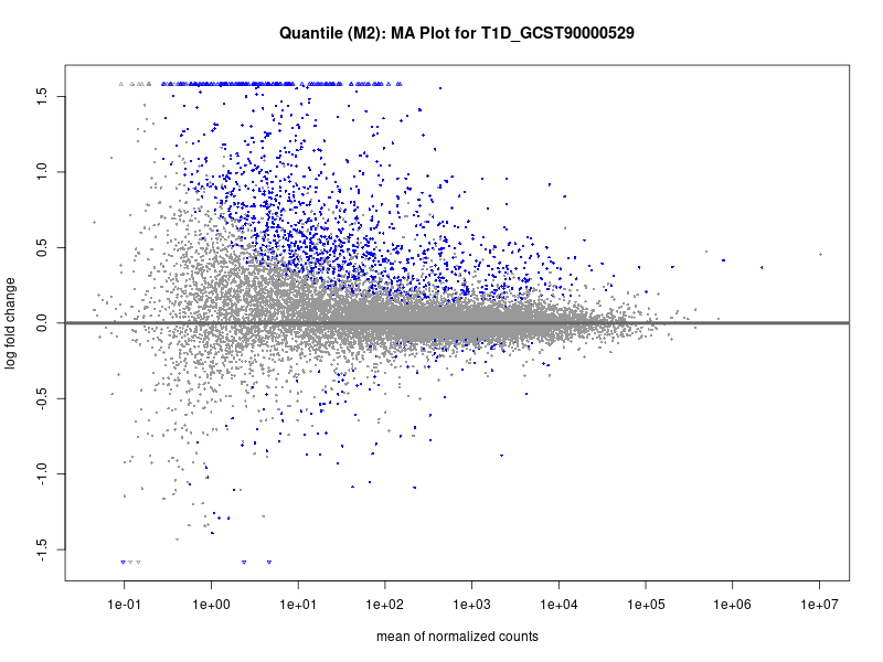
  # plot the MA-plot for the current trait
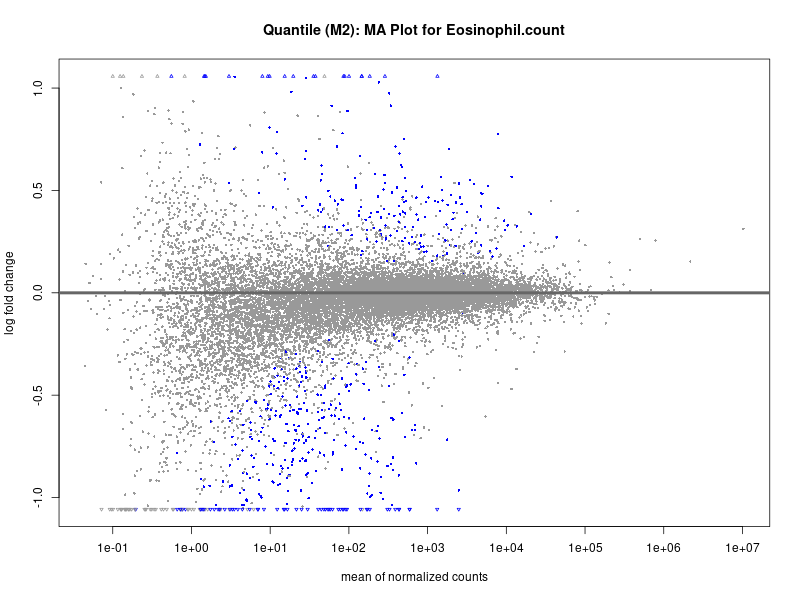
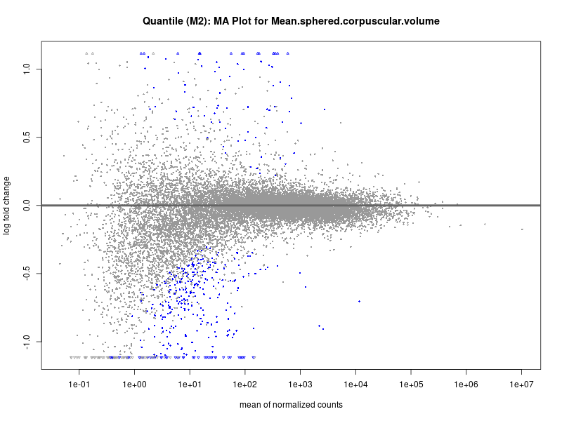
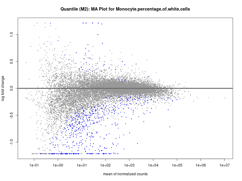
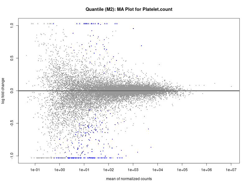
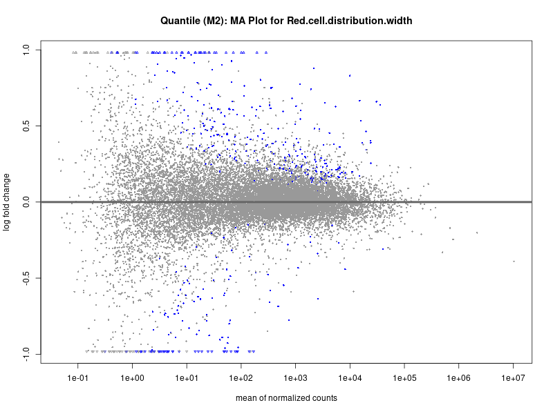
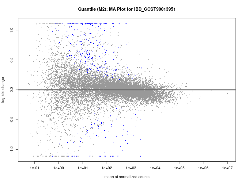
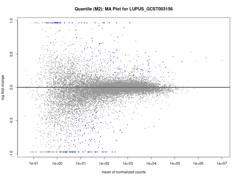
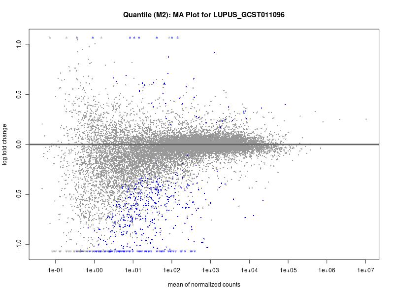
  png(paste0("ma_plot_quantile_", trait, "_M2.png"), width = 800, height = 600)
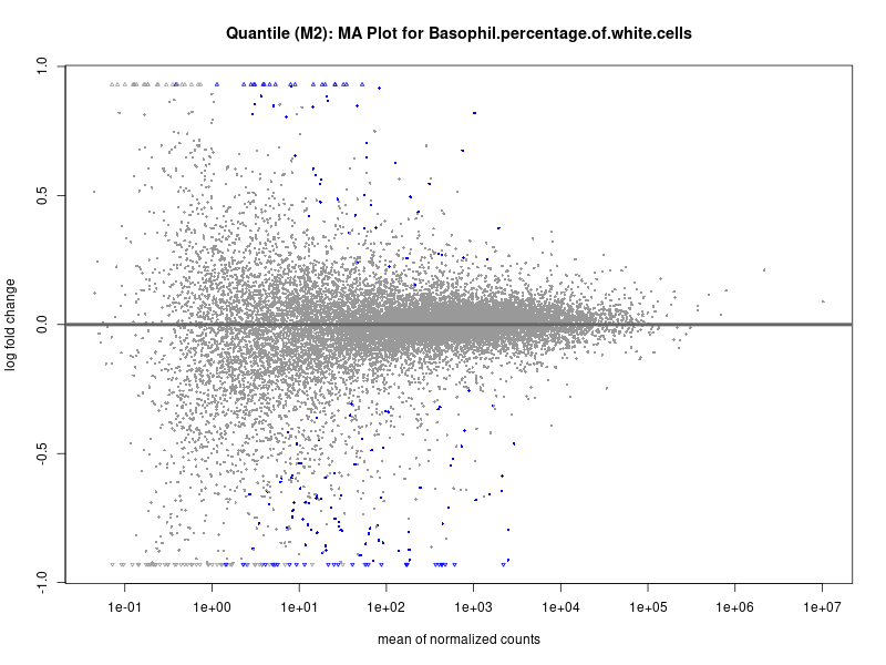
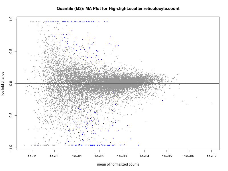
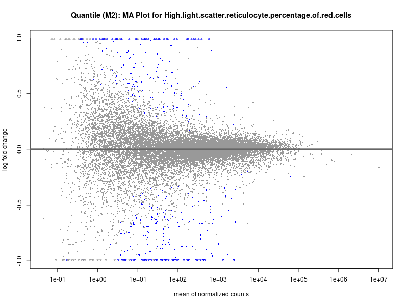
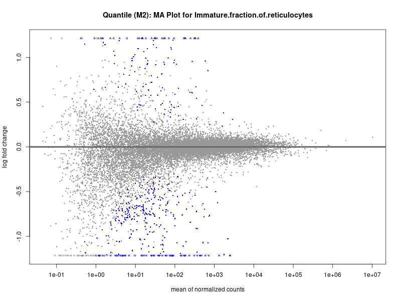
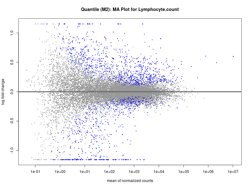
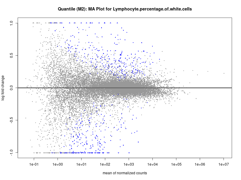
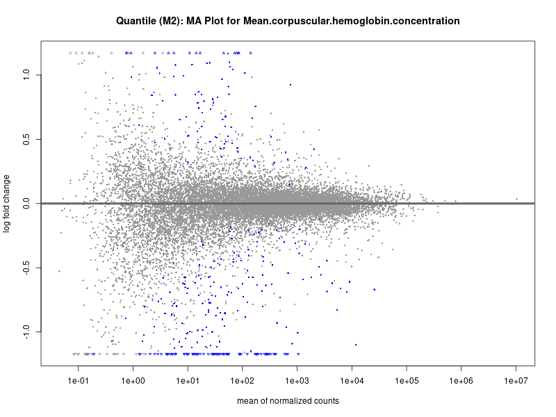
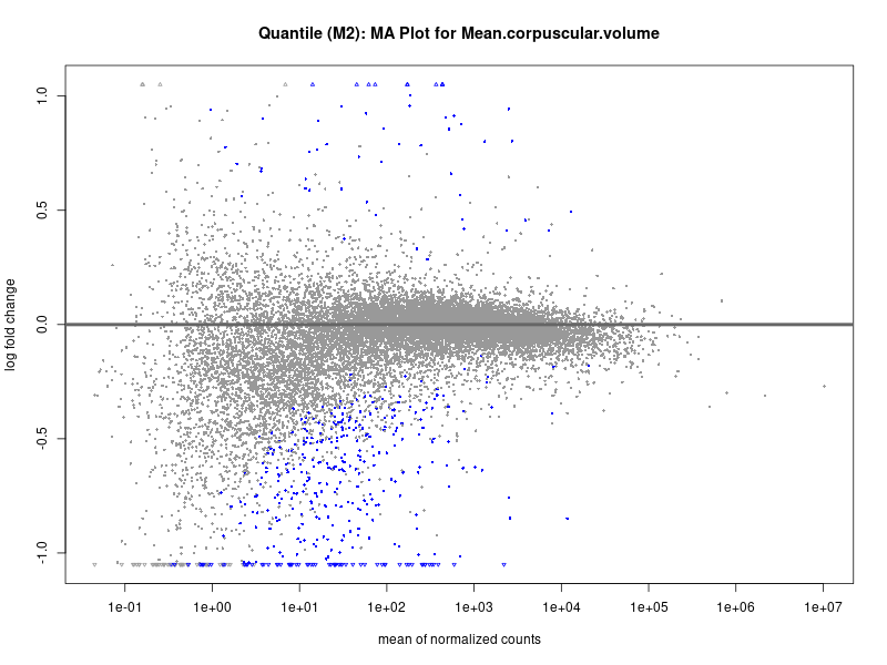
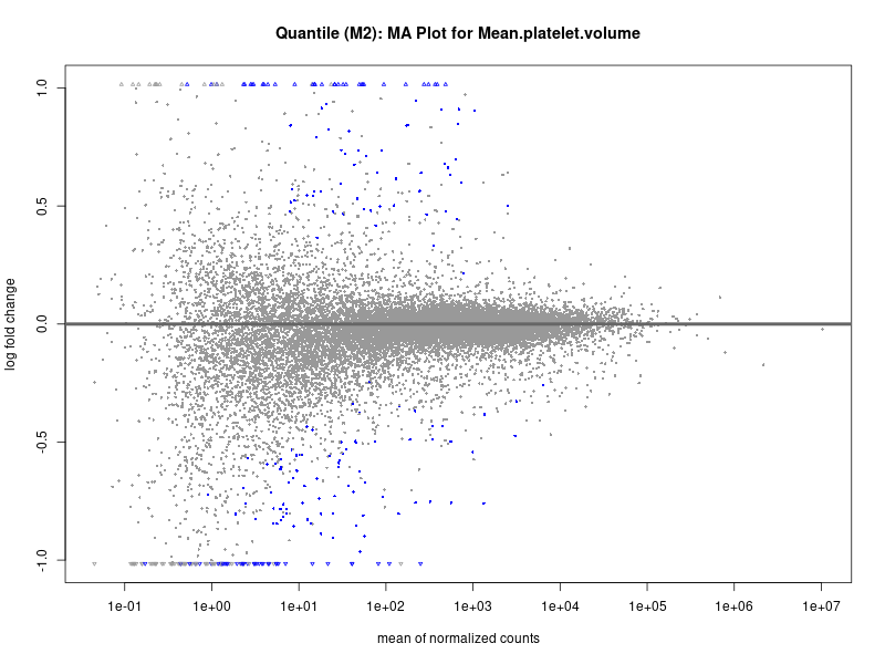
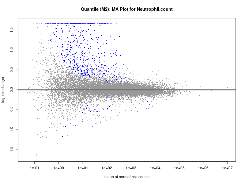
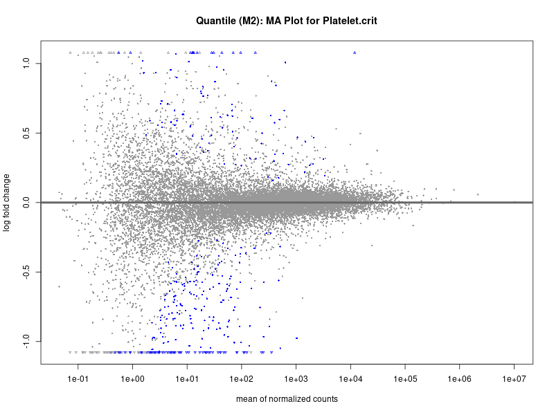
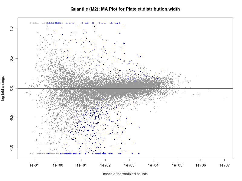
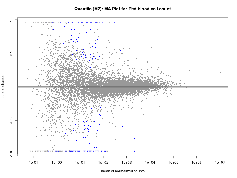
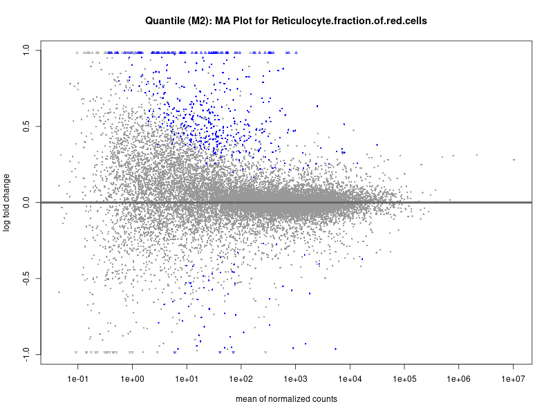
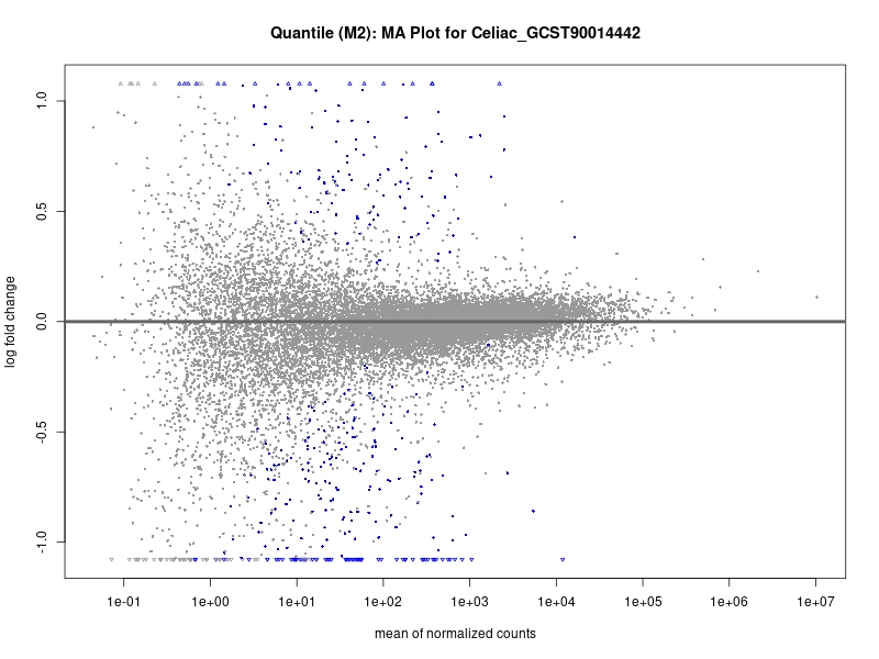
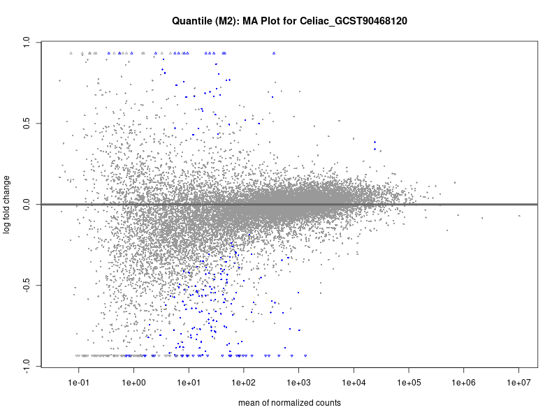
  plotMA(res, main = paste("Quantile (M2): MA Plot for", trait))
  dev.off()
  
  # volcano plot
  res_tableOE <- as.data.frame(res)
  res_tableOE$gene_name <- raw_count_df$Description[keep_genes]
  res_tableOE <- mutate(res_tableOE, threshold_OE = padj < 0.1 & 
                          abs(log2FoldChange) >= 0.5)
  res_tableOE <- res_tableOE %>% arrange(padj) %>% mutate(genelabels = "")
  res_tableOE$genelabels[1:10] <- res_tableOE$gene_name[1:10]
  
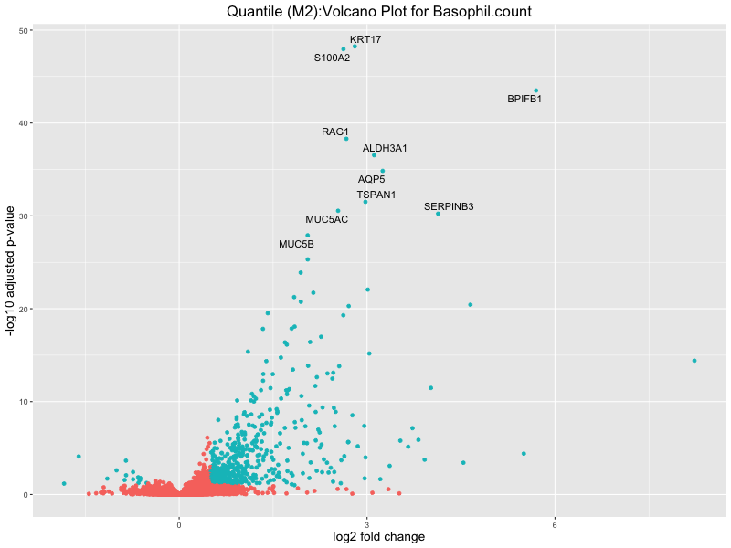
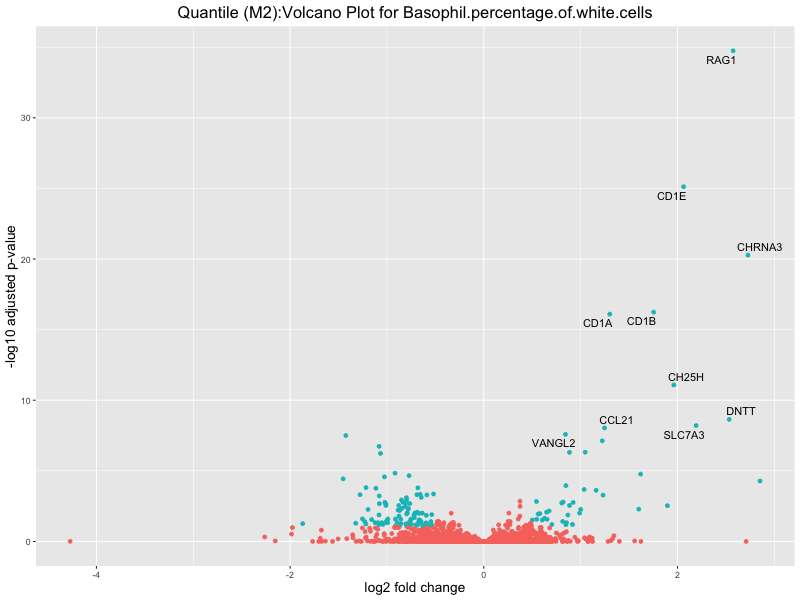
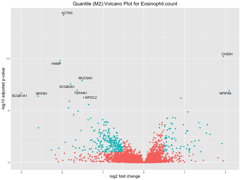
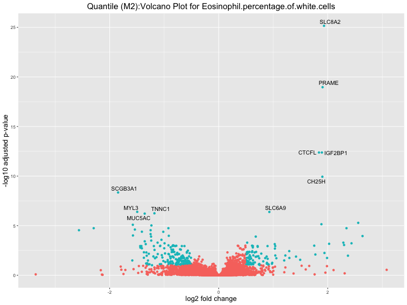
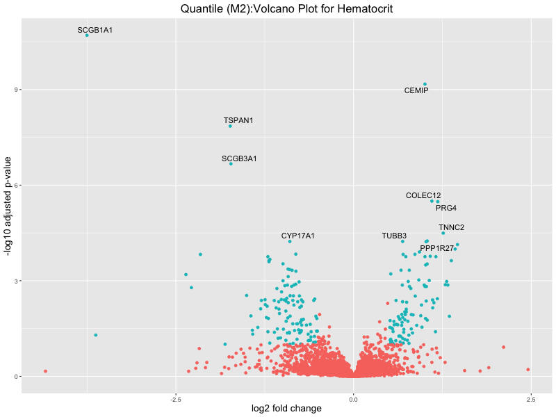
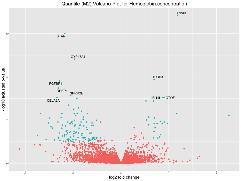
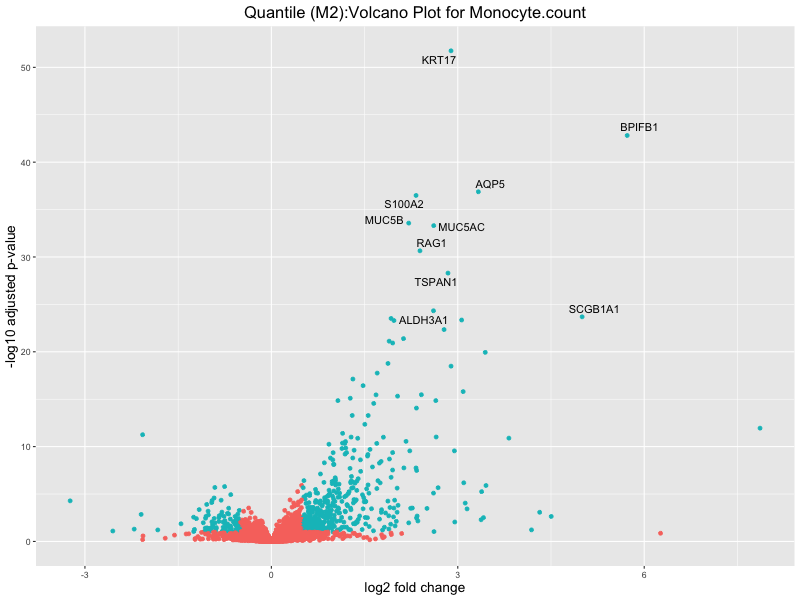
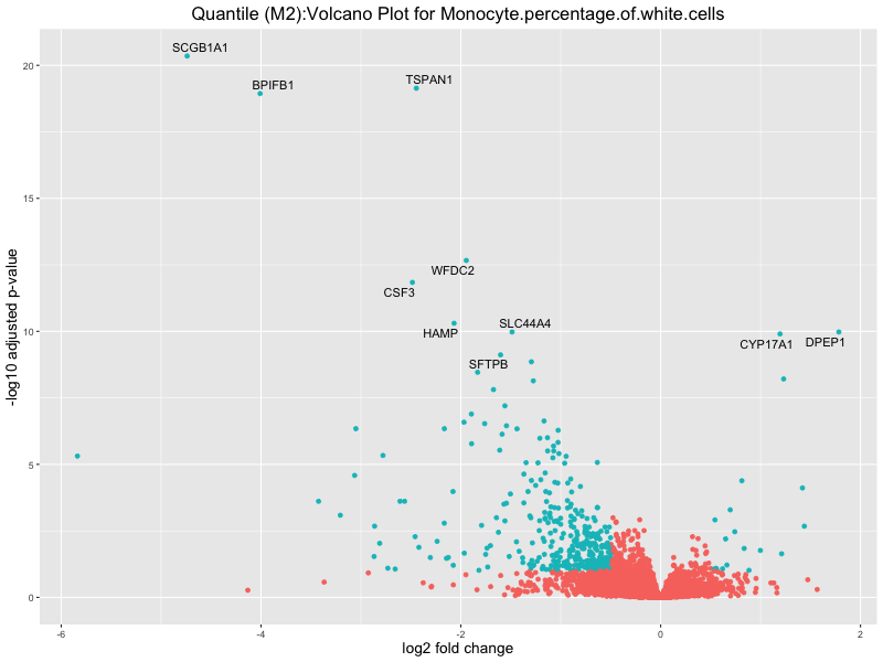
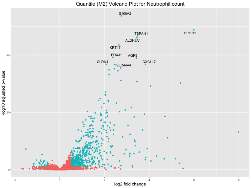
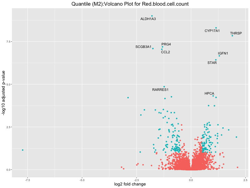
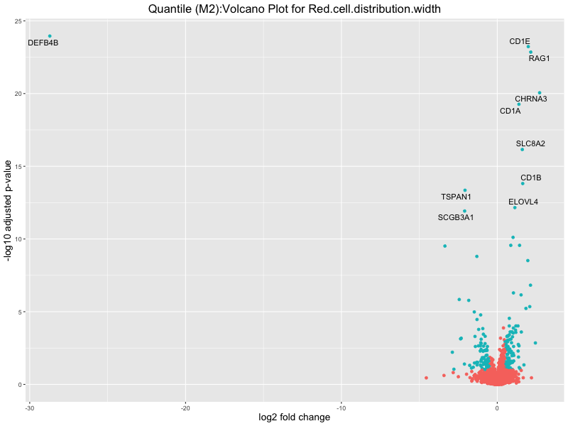
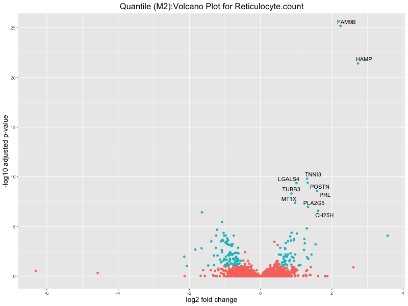
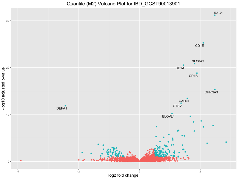
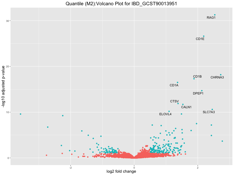
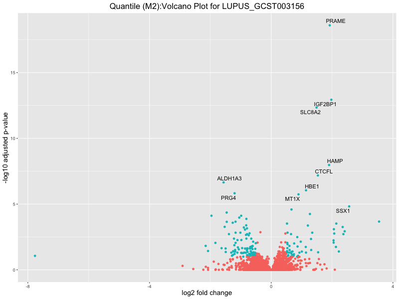
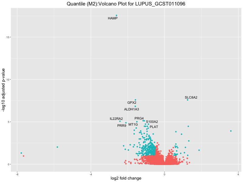
  volcano_plot <- ggplot(res_tableOE, aes(x = log2FoldChange, y = -log10(padj))) +
    geom_point(aes(colour = threshold_OE)) +
    geom_text_repel(aes(label = genelabels)) +
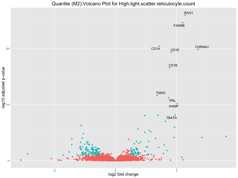
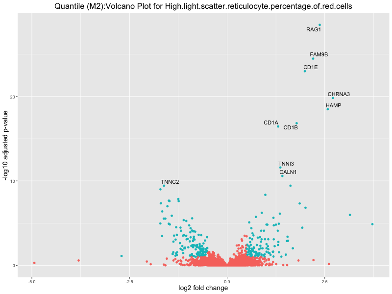
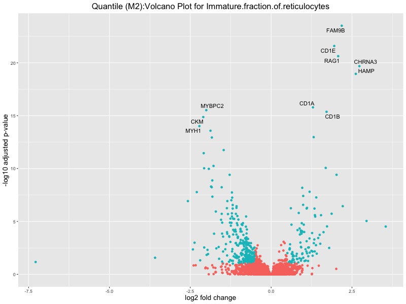
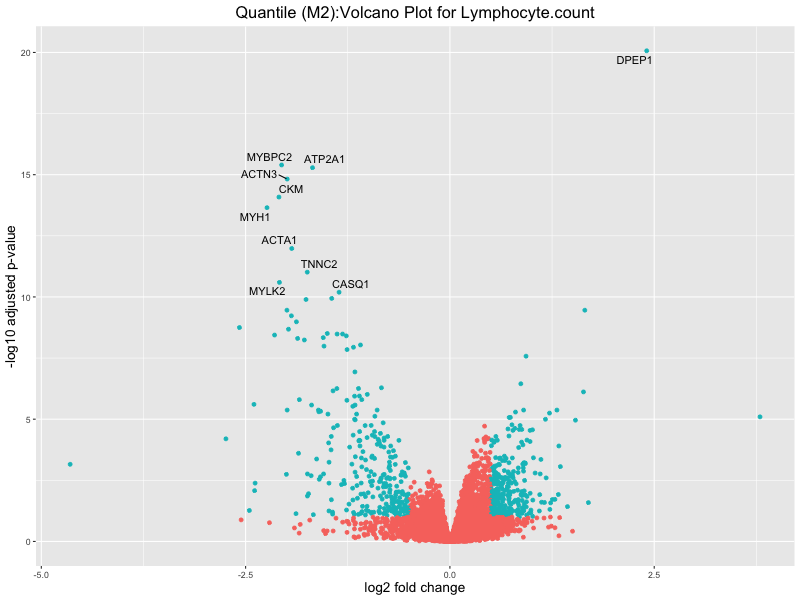
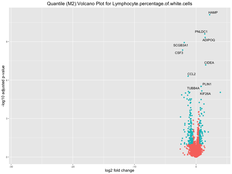
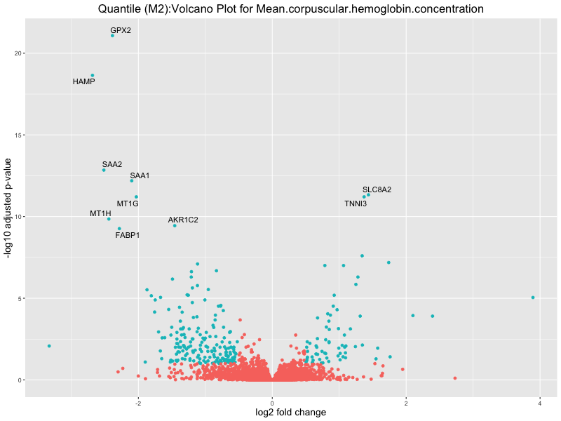
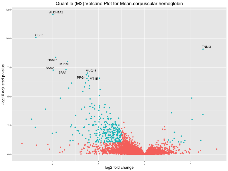
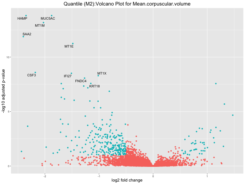
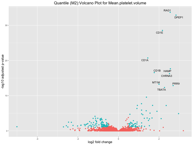
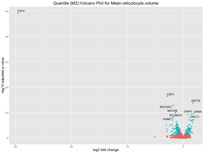
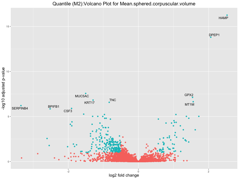
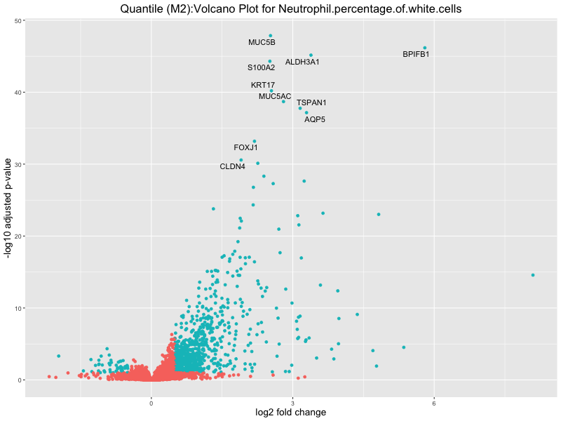
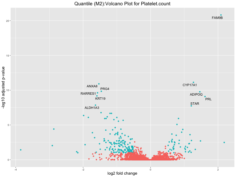
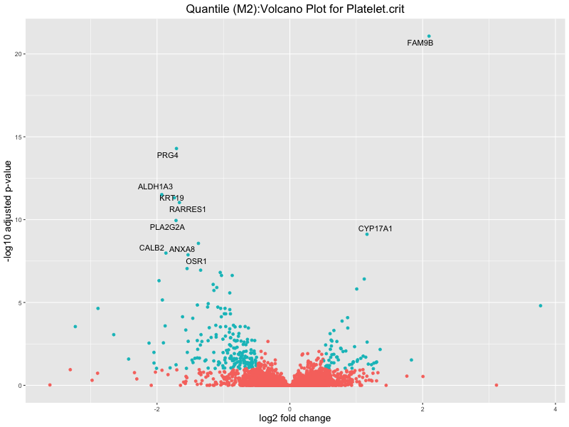
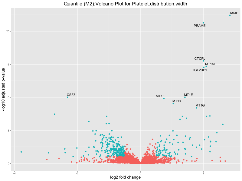
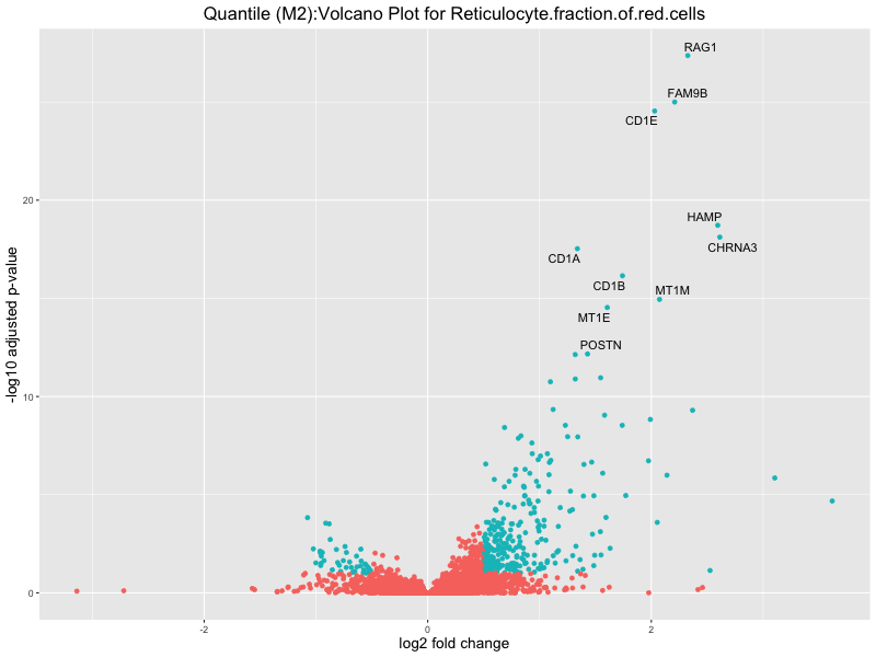
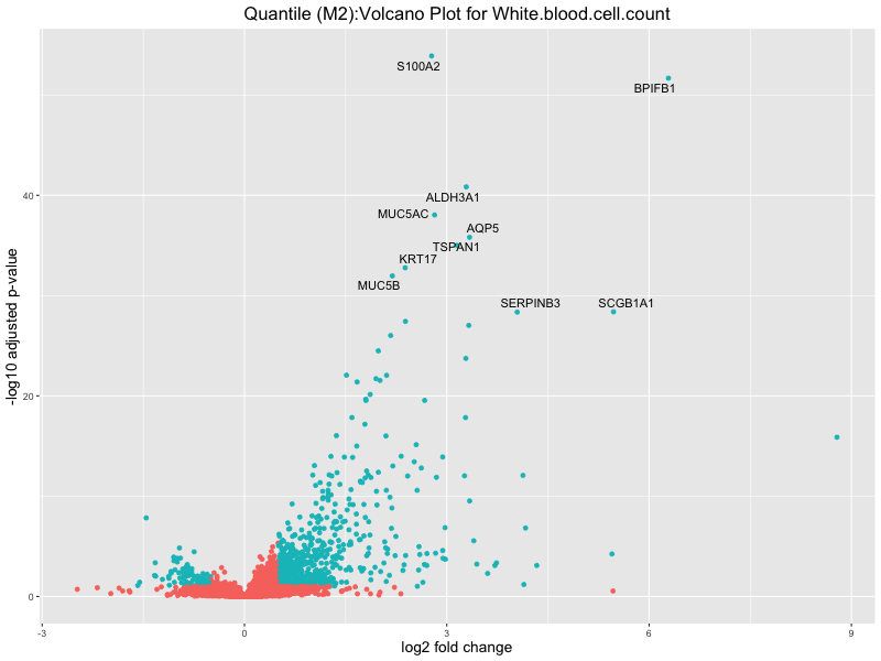
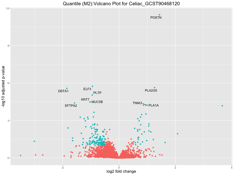
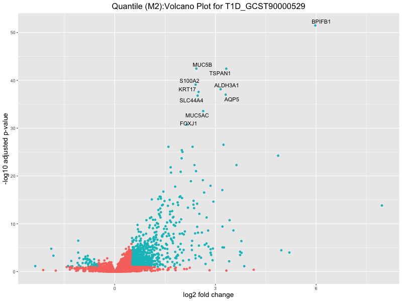
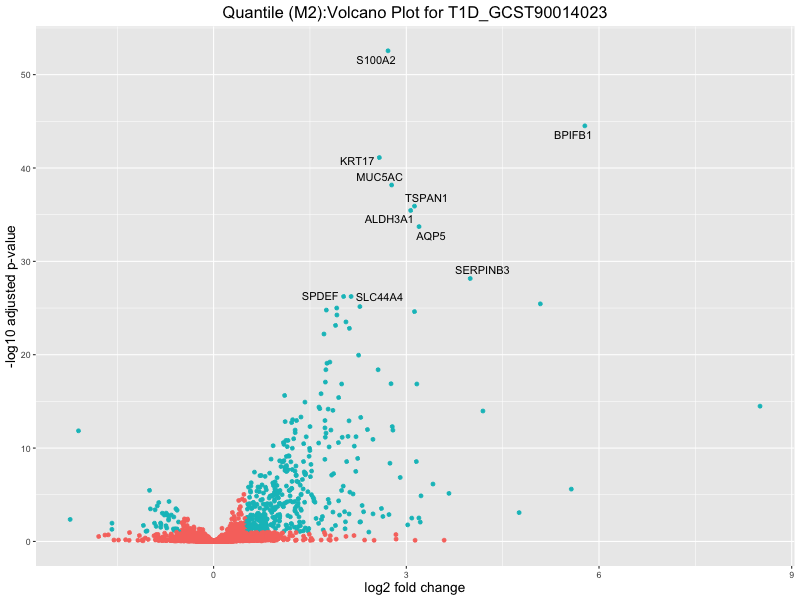
    ggtitle(paste("Quantile (M2):Volcano Plot for", trait)) +
    xlab("log2 fold change") + 
    ylab("-log10 adjusted p-value") +
    theme(legend.position = "none",
          plot.title = element_text(size = rel(1.5), hjust = 0.5),
          axis.title = element_text(size = rel(1.25)))
  
  # Save the volcano plot
  png(paste0("volcano_plot_quantile_", trait, "_M2.png"), width = 800, height = 600)
  print(volcano_plot)
  dev.off()
}

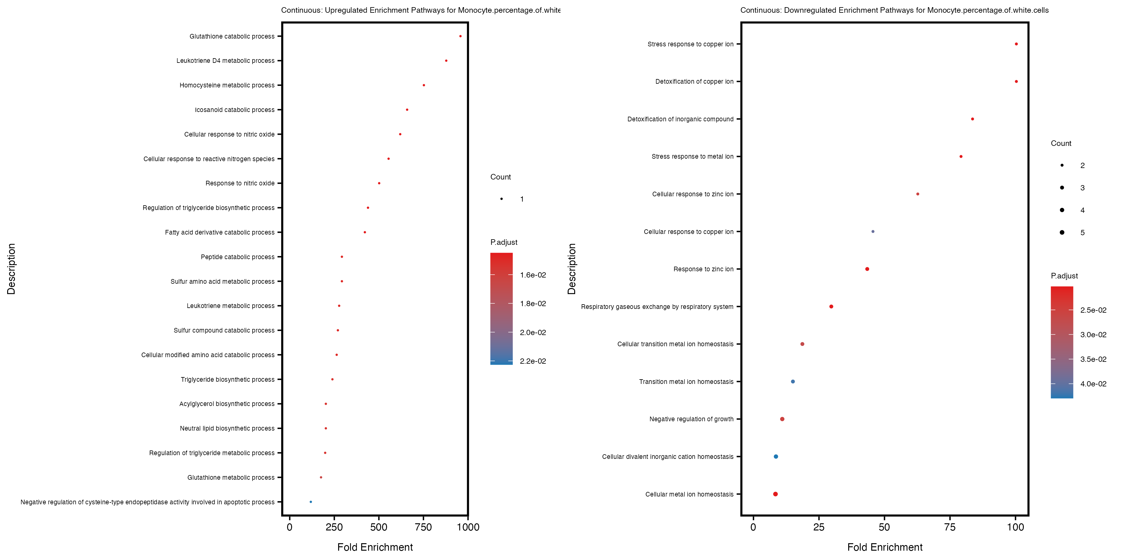
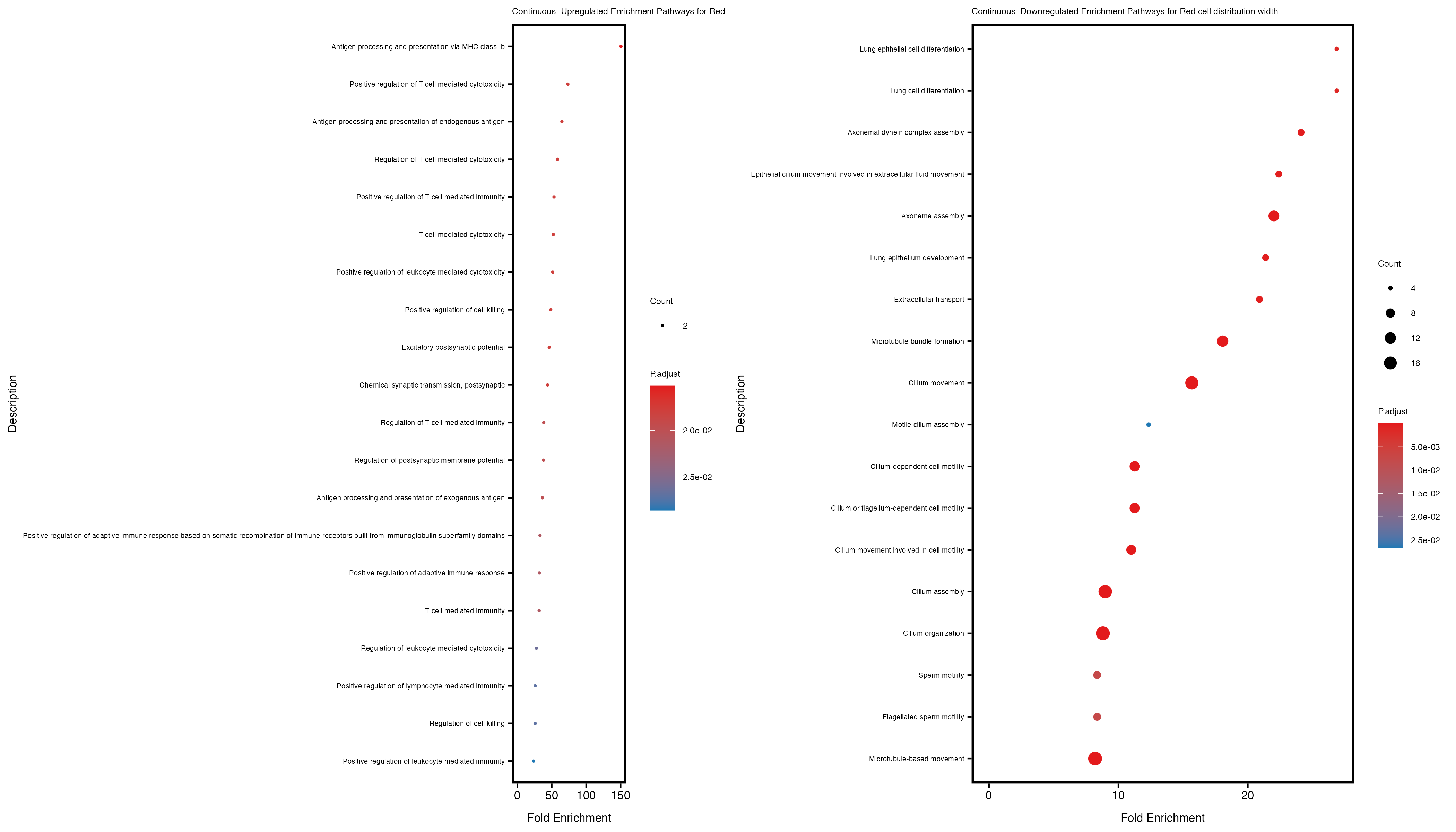
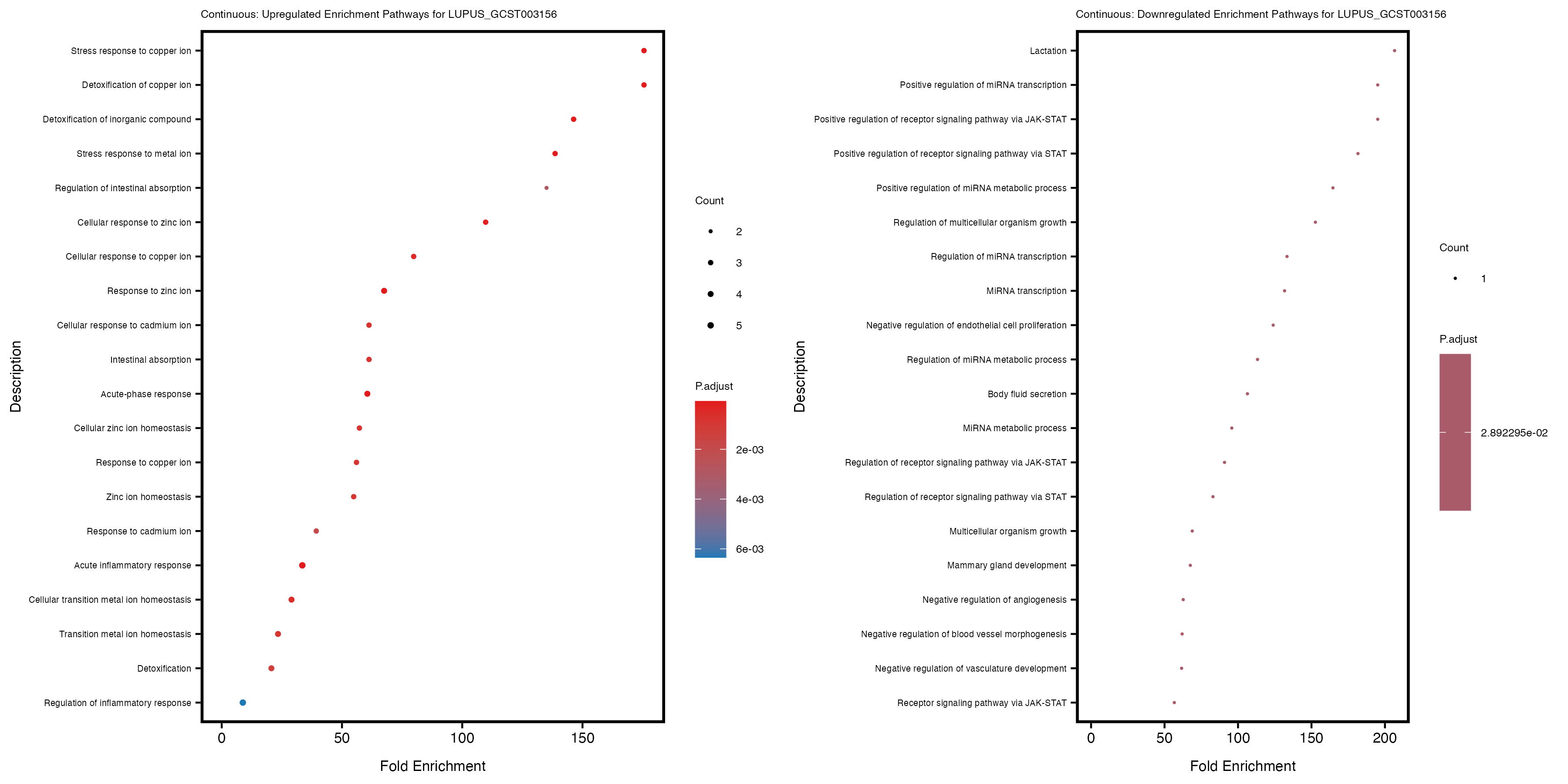
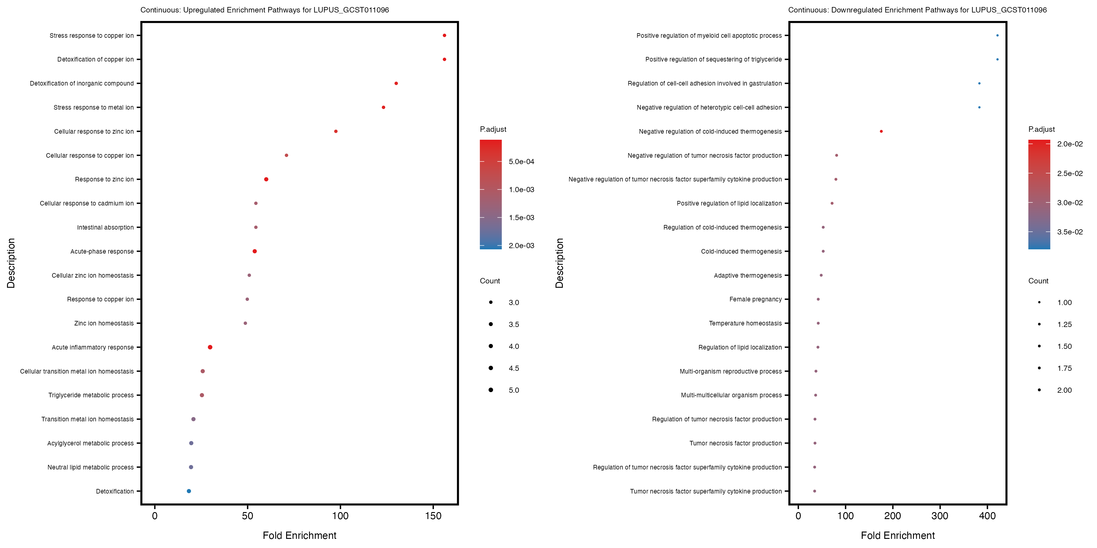
GO enrichment Analysis

Gene Ontology enrichment is applied to both models, with and without adjusting 2 genotype PCs, for both continuous & quantile PRS.

Continuous PRS:

dir_path <- "analysis/continuous_wb"
files <- list.files(dir_path, pattern = "differential_expression_.*_results.csv", 
                    full.names = TRUE)

for (file in files) {
  trait <- gsub("differential_expression_(.*)_results.csv", "\\1", basename(file))
  trait
  res_tableOE <- read.csv(file, header = T, row.names = 1)
  
  deGenes <- res_tableOE[res_tableOE$padj < 0.1 & 
                           abs(res_tableOE$log2FoldChange) >= 0.5, ]
  deGenes$gene_id <- gsub("\\.\\d+$", "", rownames(deGenes))
  
  # Separate upregulated and downregulated genes
  upregulated_genes <- deGenes[deGenes$log2FoldChange > 0, ]$gene_id
  downregulated_genes <- deGenes[deGenes$log2FoldChange < 0, ]$gene_id
  
  # Run GO enrichment for upregulated genes
  gse_up <- enrichGO(gene = upregulated_genes, ont = "BP", 
                   OrgDb = "org.Hs.eg.db", keyType = "ENSEMBL", readable = T)
  
  # Run GO enrichment for downregulated genes
  gse_down <- enrichGO(gene = downregulated_genes, ont = "BP", 
                     OrgDb = "org.Hs.eg.db", keyType = "ENSEMBL", readable = T)
  
  # Convert enrichment results to data frames and calculate additional ratios
  if (is.null(gse_up)) {
    gse_up <- data.frame(ID = character(), Description = character(),
                       GeneRatio = character(), BgRatio = character(),
                       pvalue = numeric(), p.adjust = numeric(),
                       qvalue = numeric(), geneID = character(),
                       Count = integer(), stringsAsFactors = FALSE)
  } else { 
    gse_up <- as.data.frame(gse_up)}
  
  gse_down <- as.data.frame(gse_down)
  
  gse_up$GeneRatio_num <- as.numeric(sapply(strsplit(gse_up$GeneRatio, "/"), function(x) x[1])) / 
                        as.numeric(sapply(strsplit(gse_up$GeneRatio, "/"), function(x) x[2]))
  gse_up$BgRatio_num <- as.numeric(sapply(strsplit(gse_up$BgRatio, "/"), function(x) x[1])) / 
                        as.numeric(sapply(strsplit(gse_up$BgRatio, "/"), function(x) x[2]))
  gse_up <- cbind(gse_up, FoldEnrich = gse_up$GeneRatio_num / gse_up$BgRatio_num)

  gse_down$GeneRatio_num <- as.numeric(sapply(strsplit(gse_down$GeneRatio, "/"), function(x) x[1])) / 
                          as.numeric(sapply(strsplit(gse_down$GeneRatio, "/"), function(x) x[2]))
  gse_down$BgRatio_num <- as.numeric(sapply(strsplit(gse_down$BgRatio, "/"), function(x) x[1])) / 
                          as.numeric(sapply(strsplit(gse_down$BgRatio, "/"), function(x) x[2]))
  gse_down <- cbind(gse_down, FoldEnrich = gse_down$GeneRatio_num / gse_down$BgRatio_num)
  
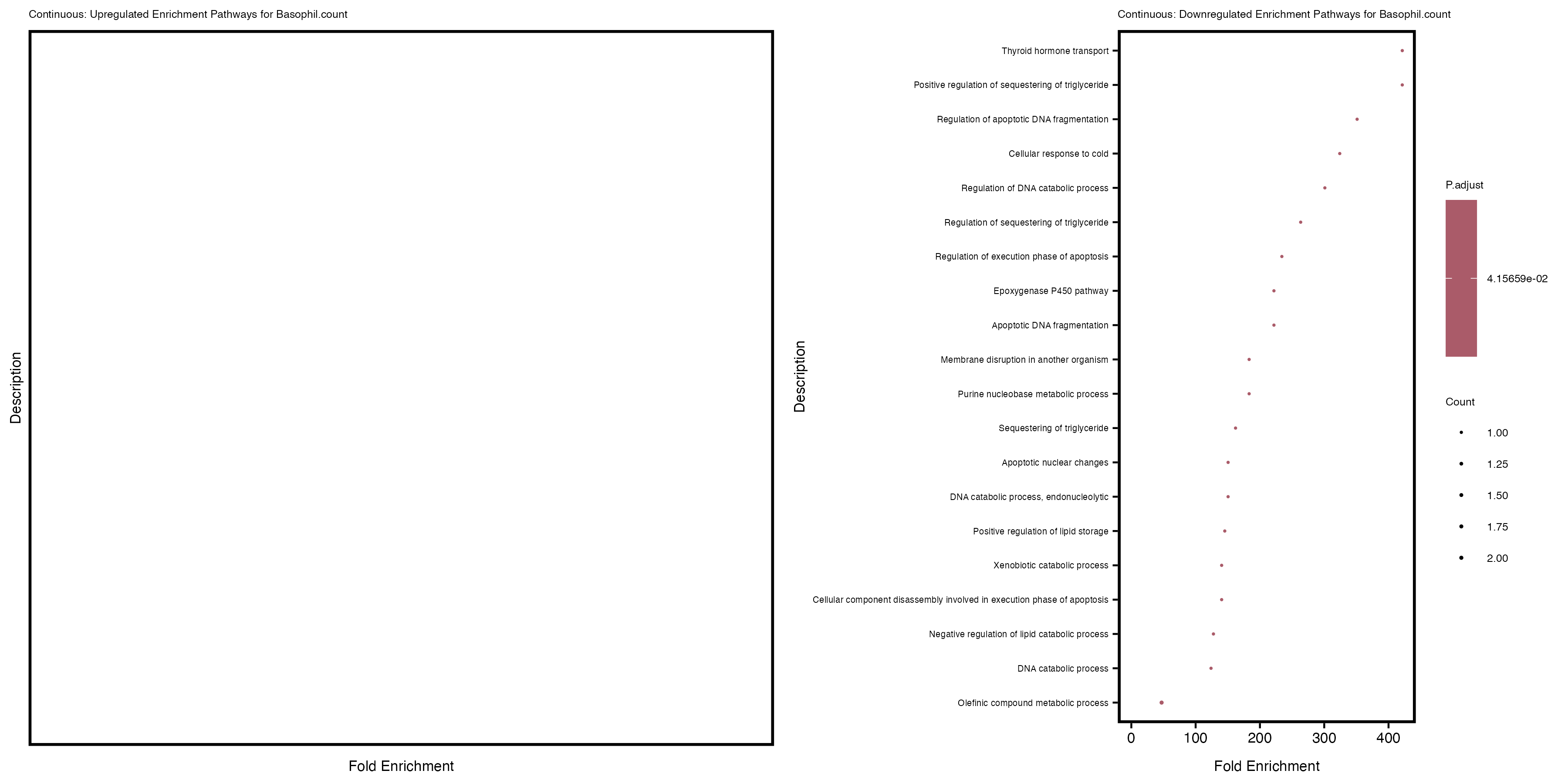
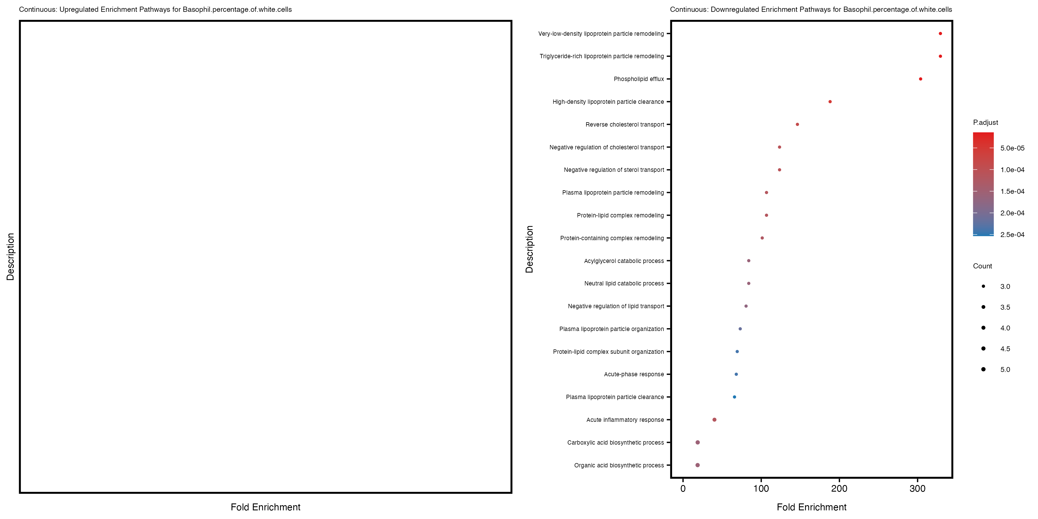
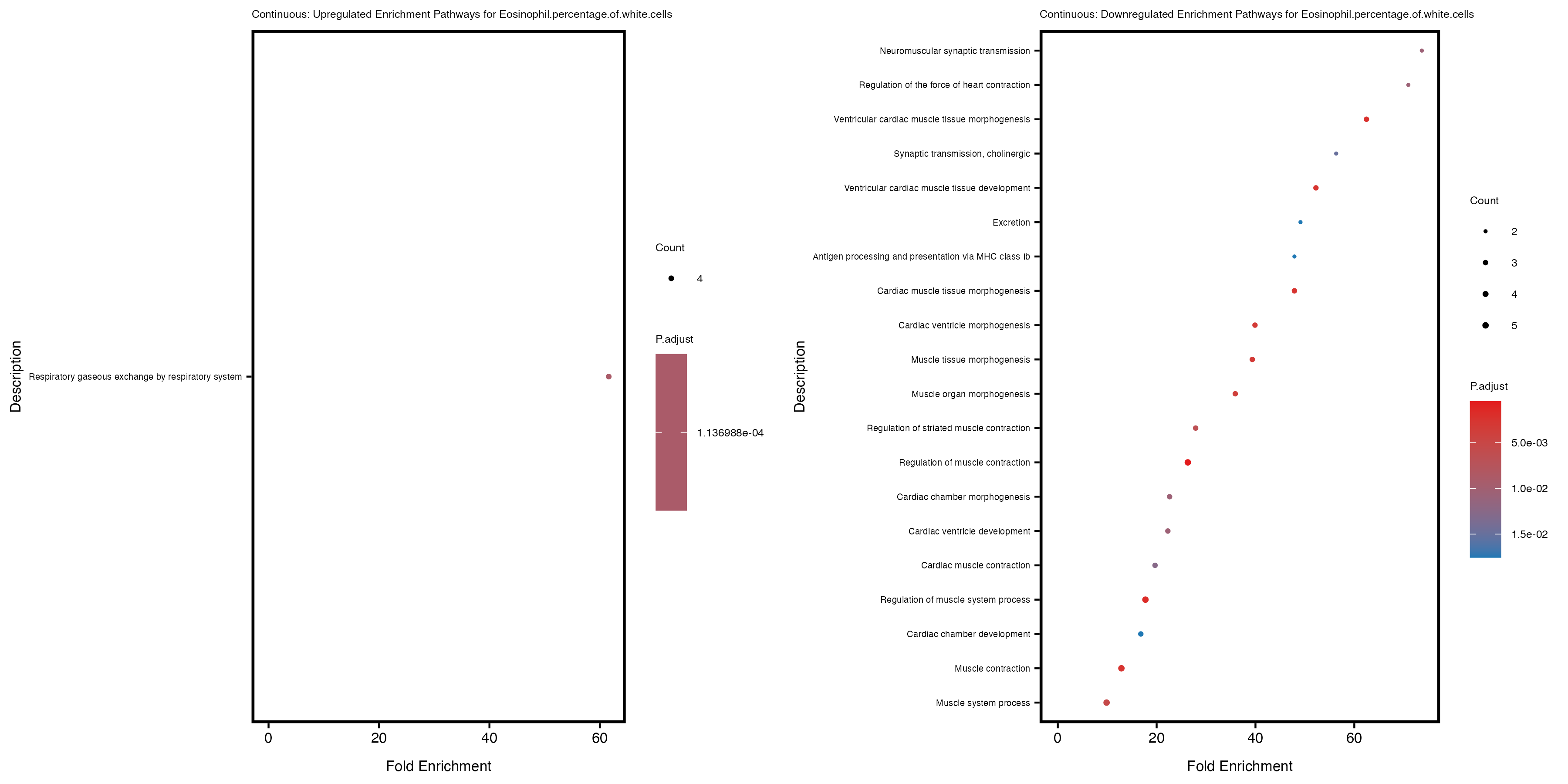
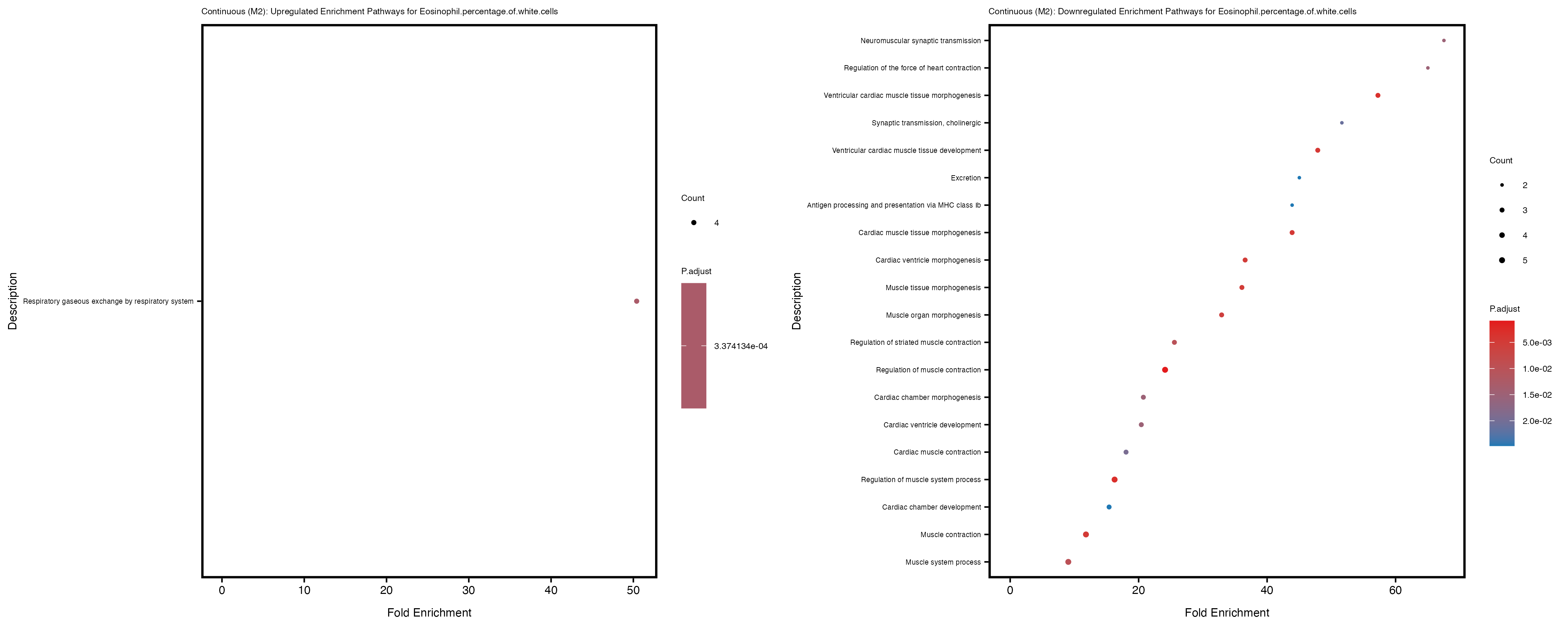
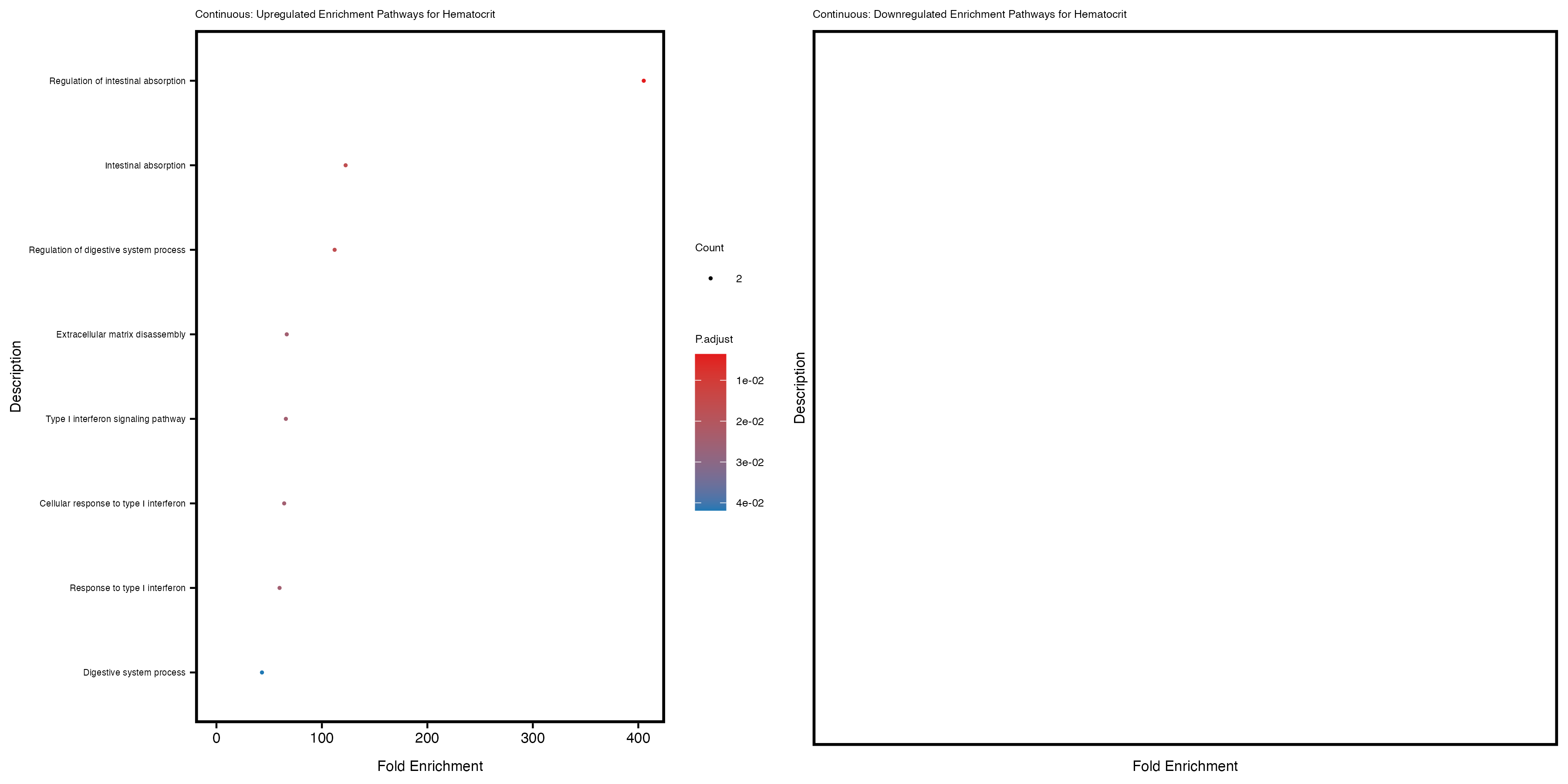
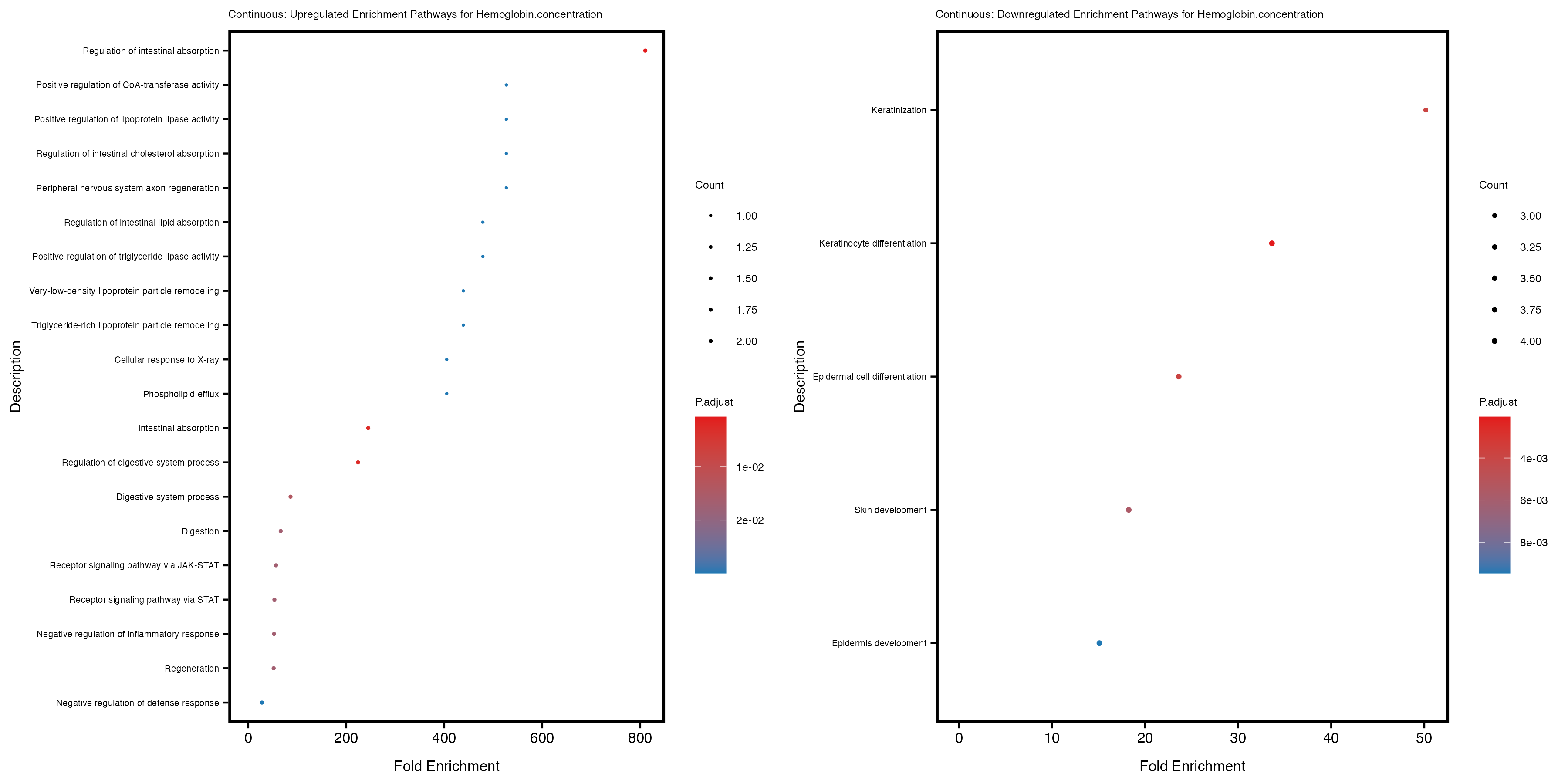
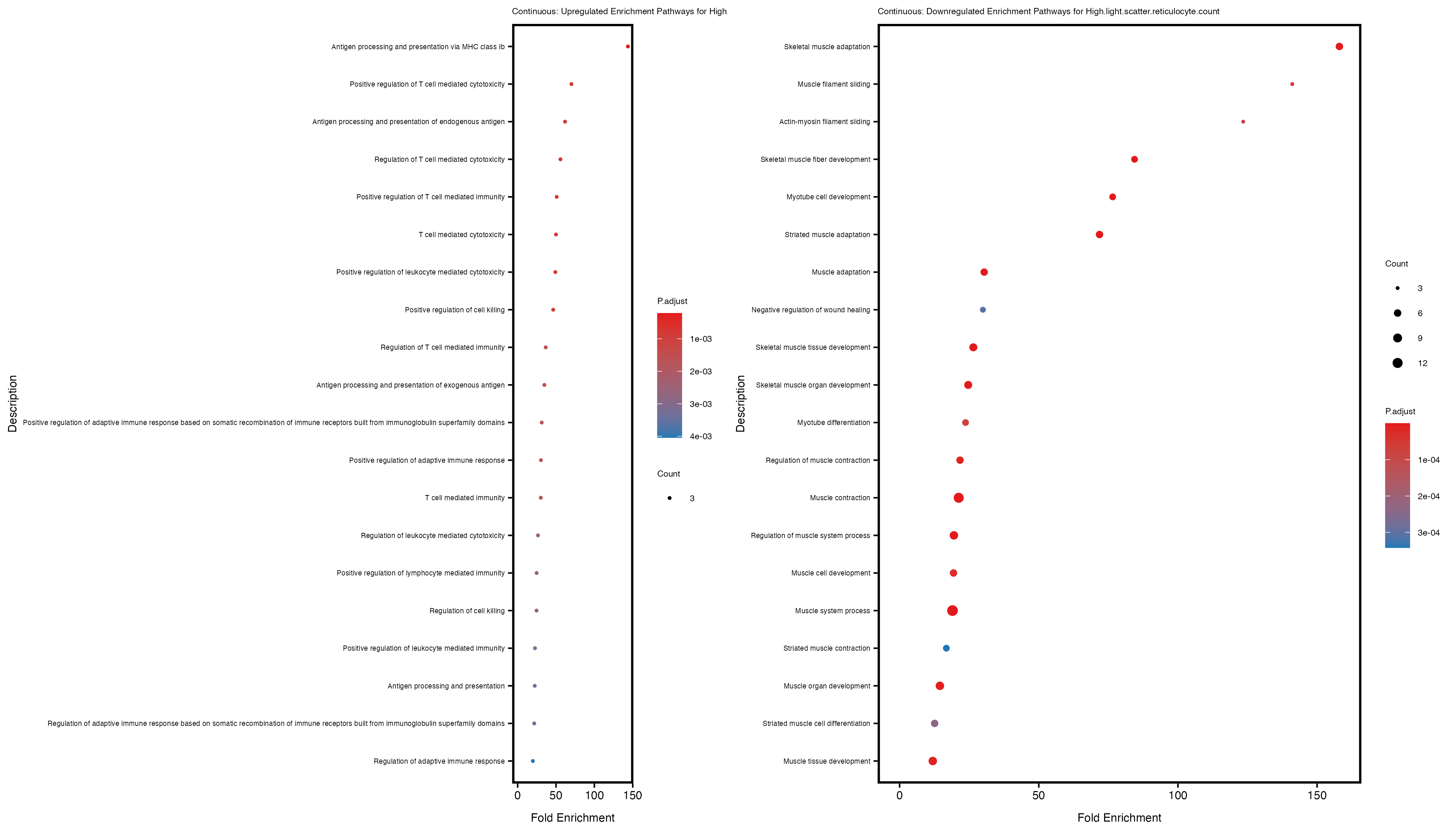
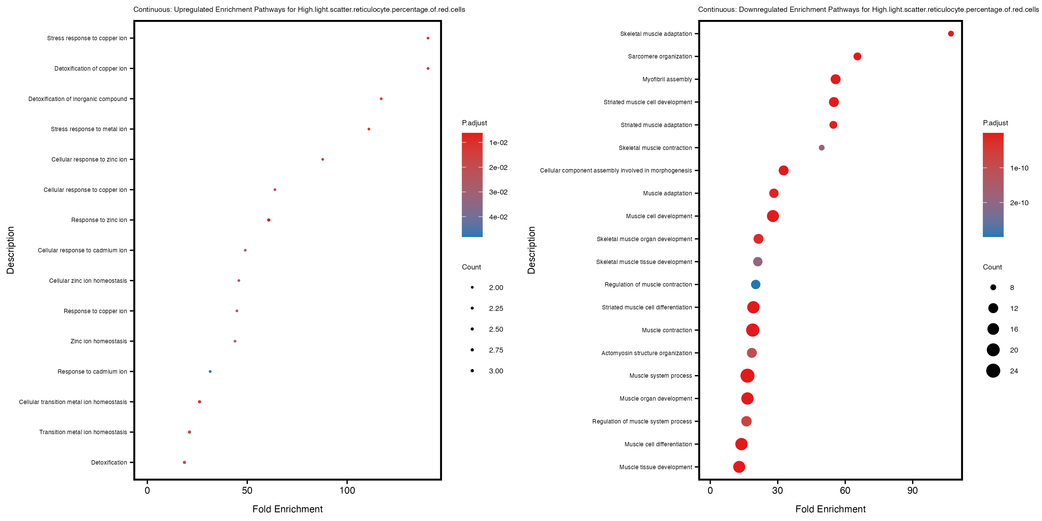
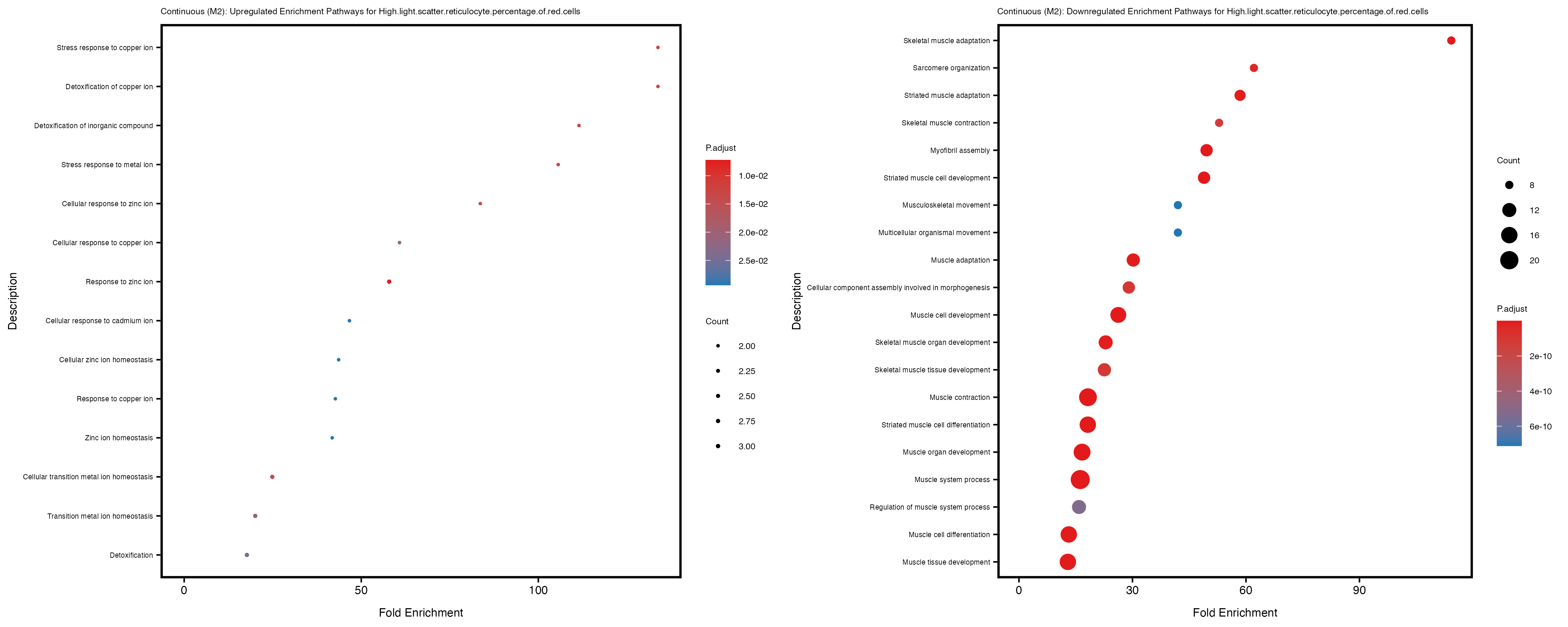
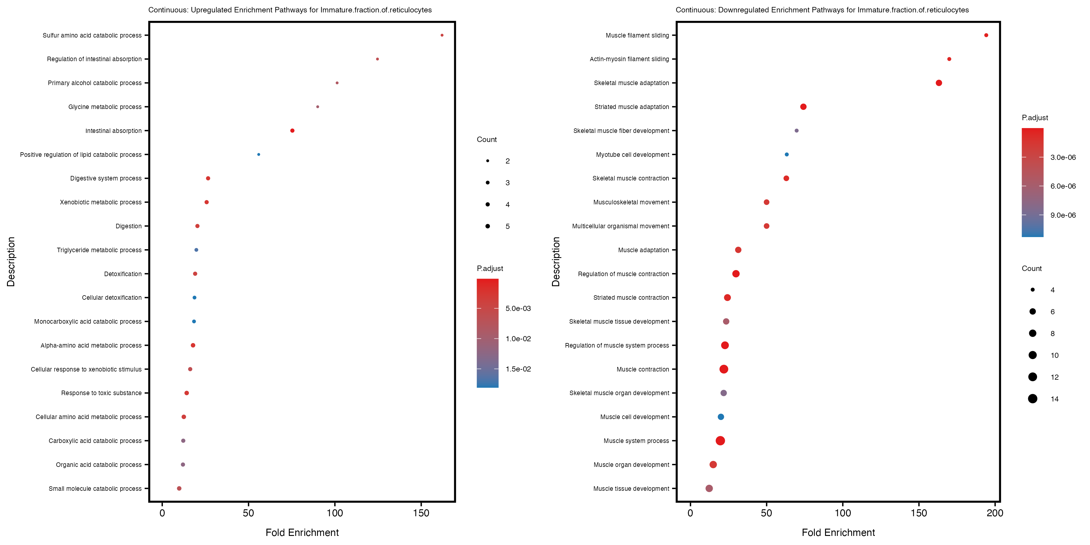
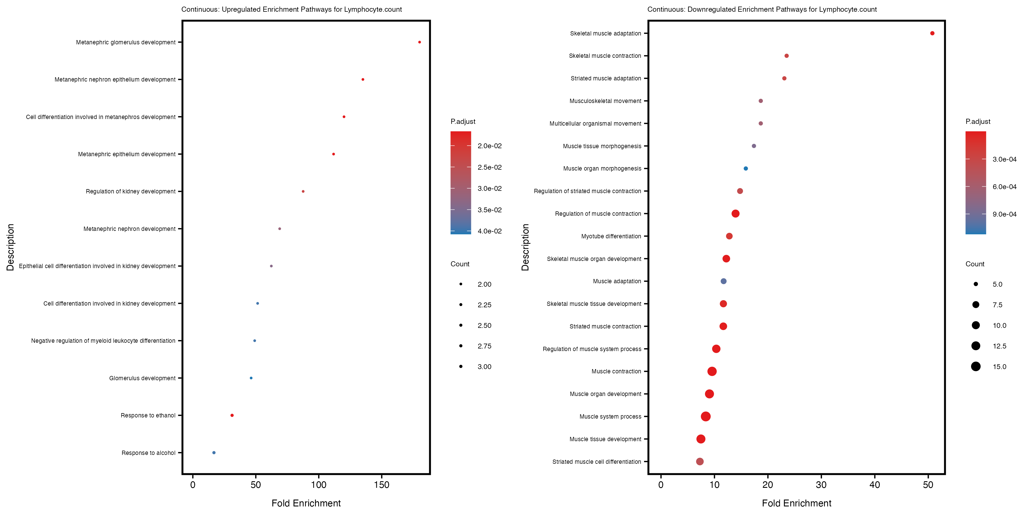
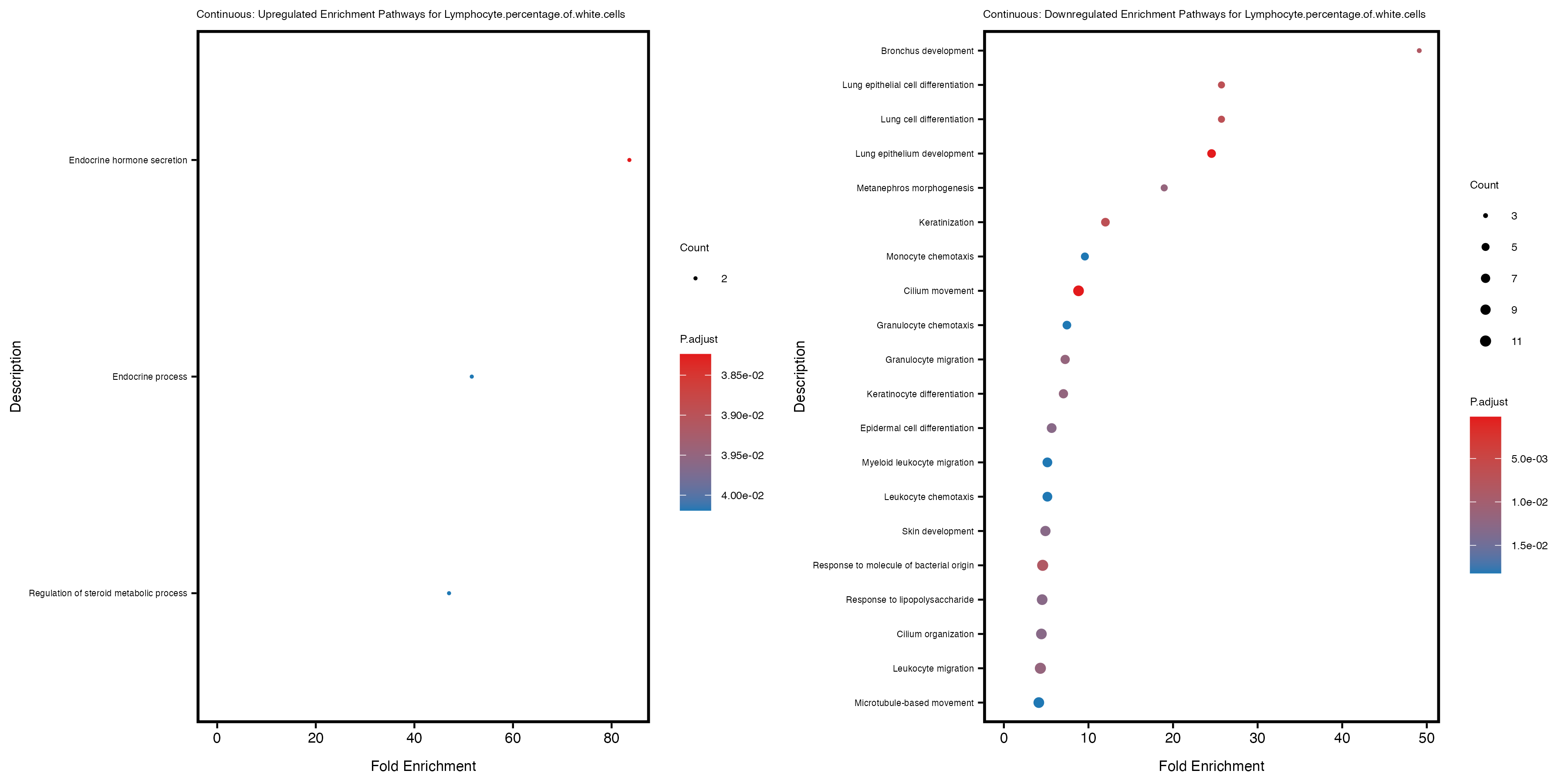
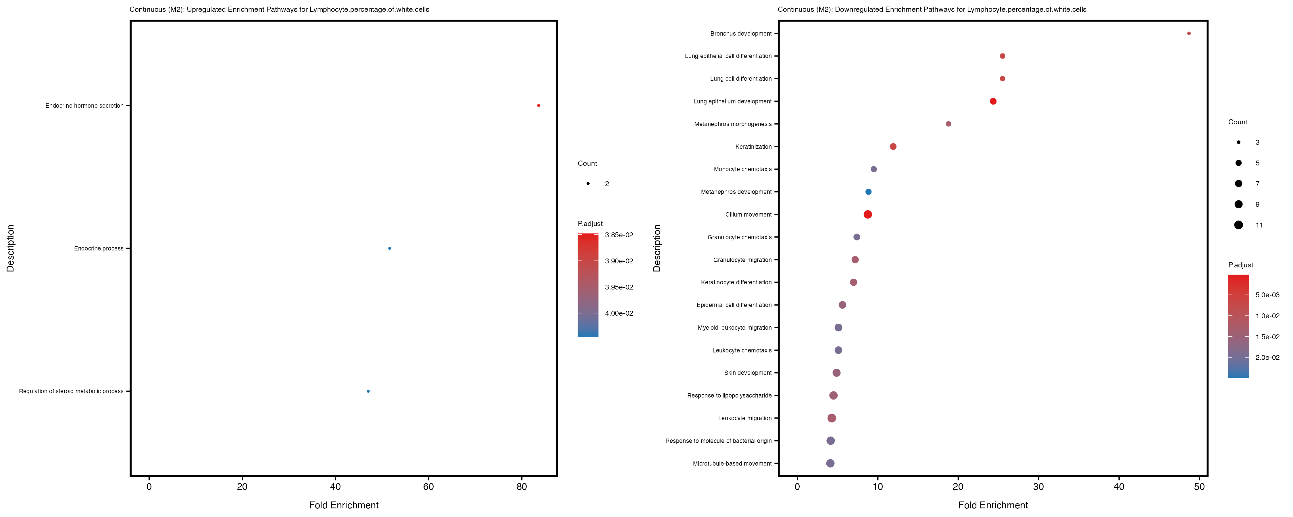
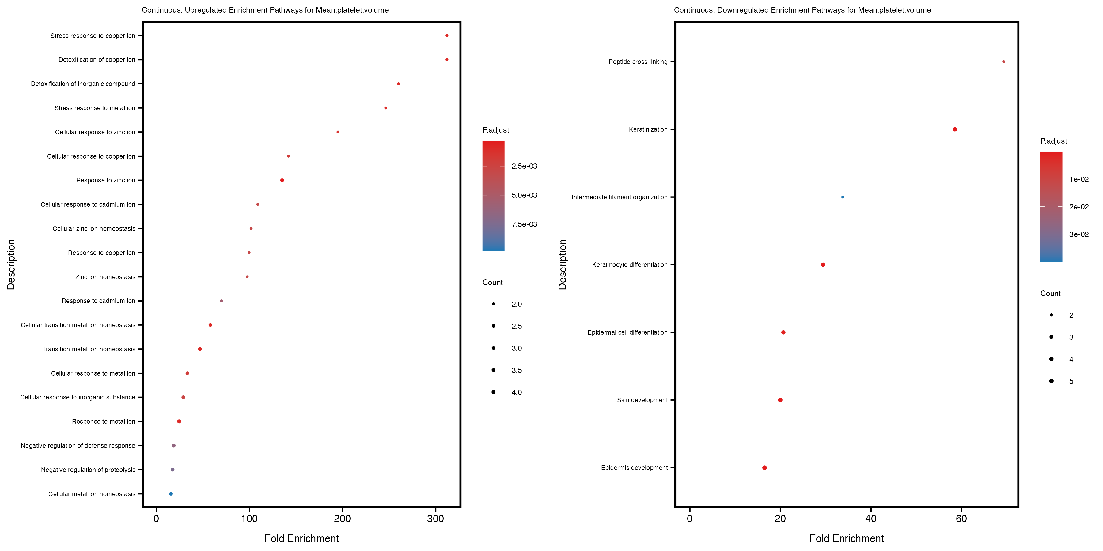
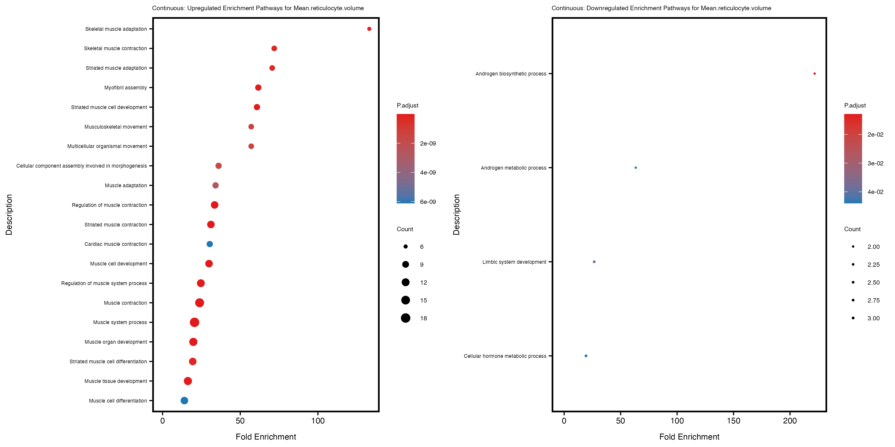
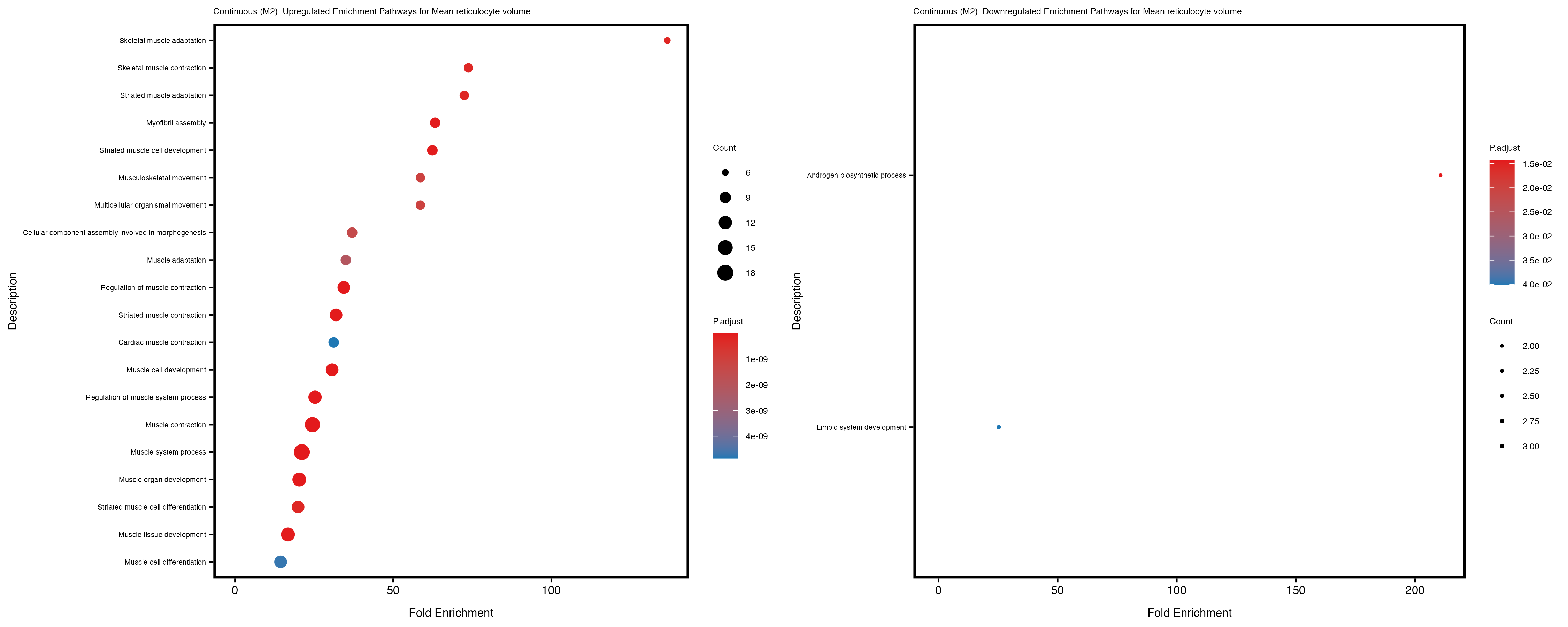
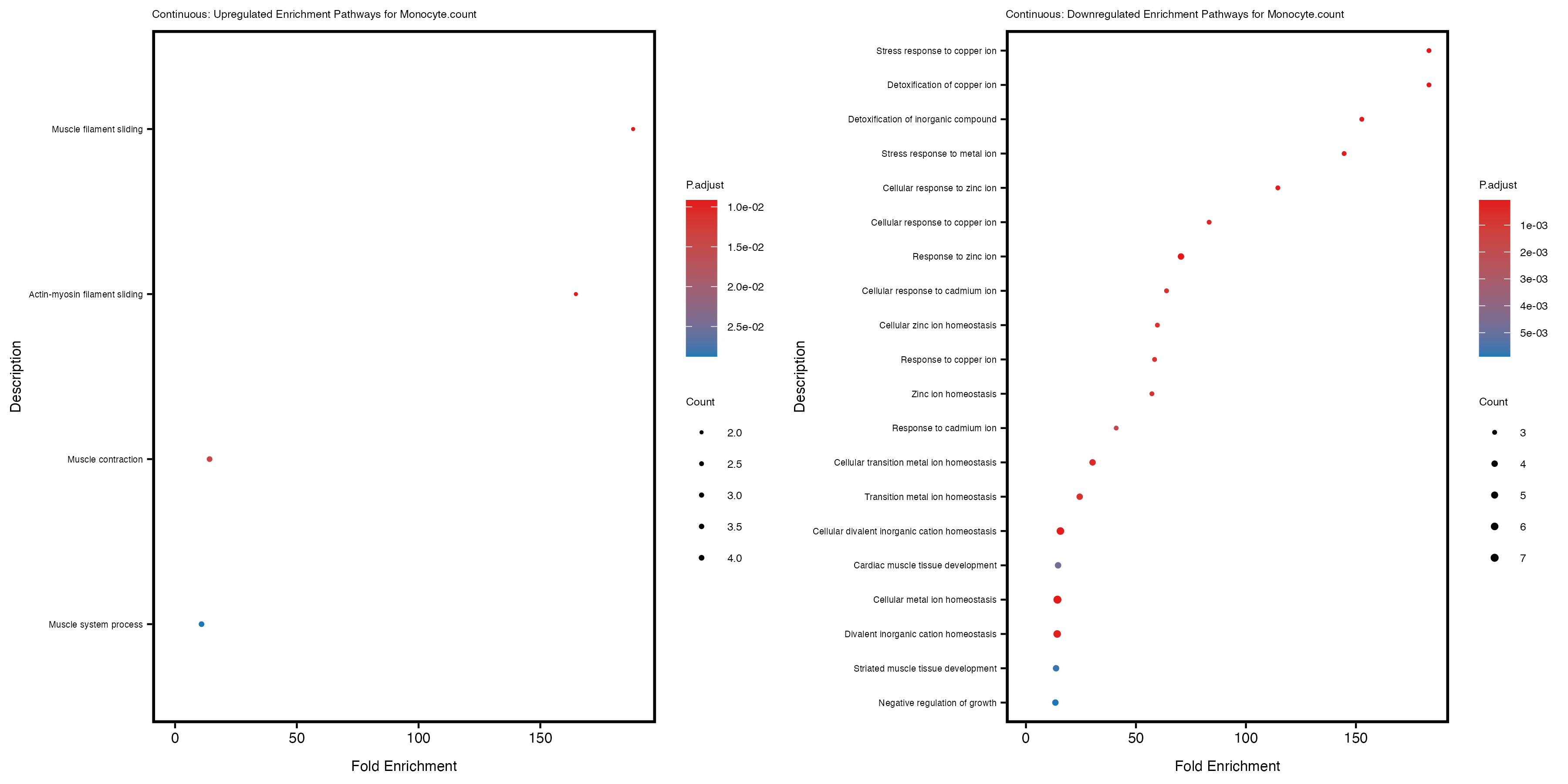
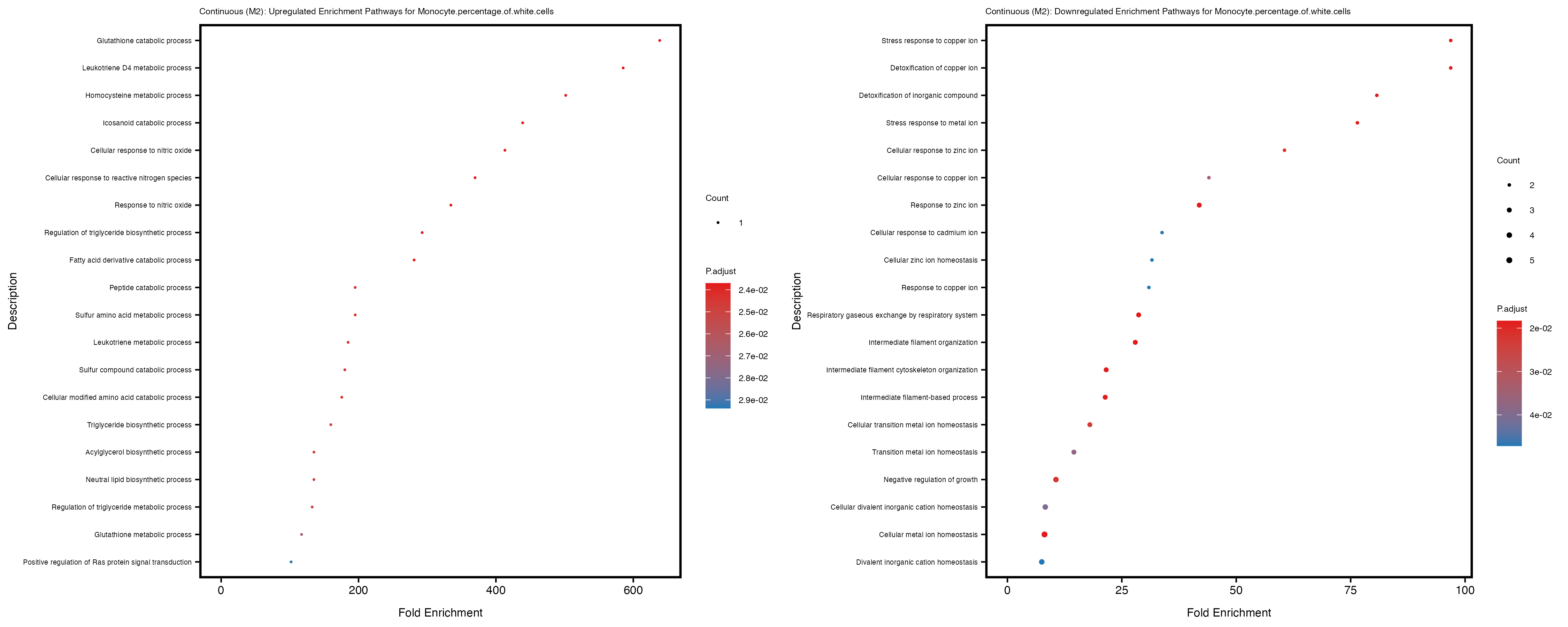
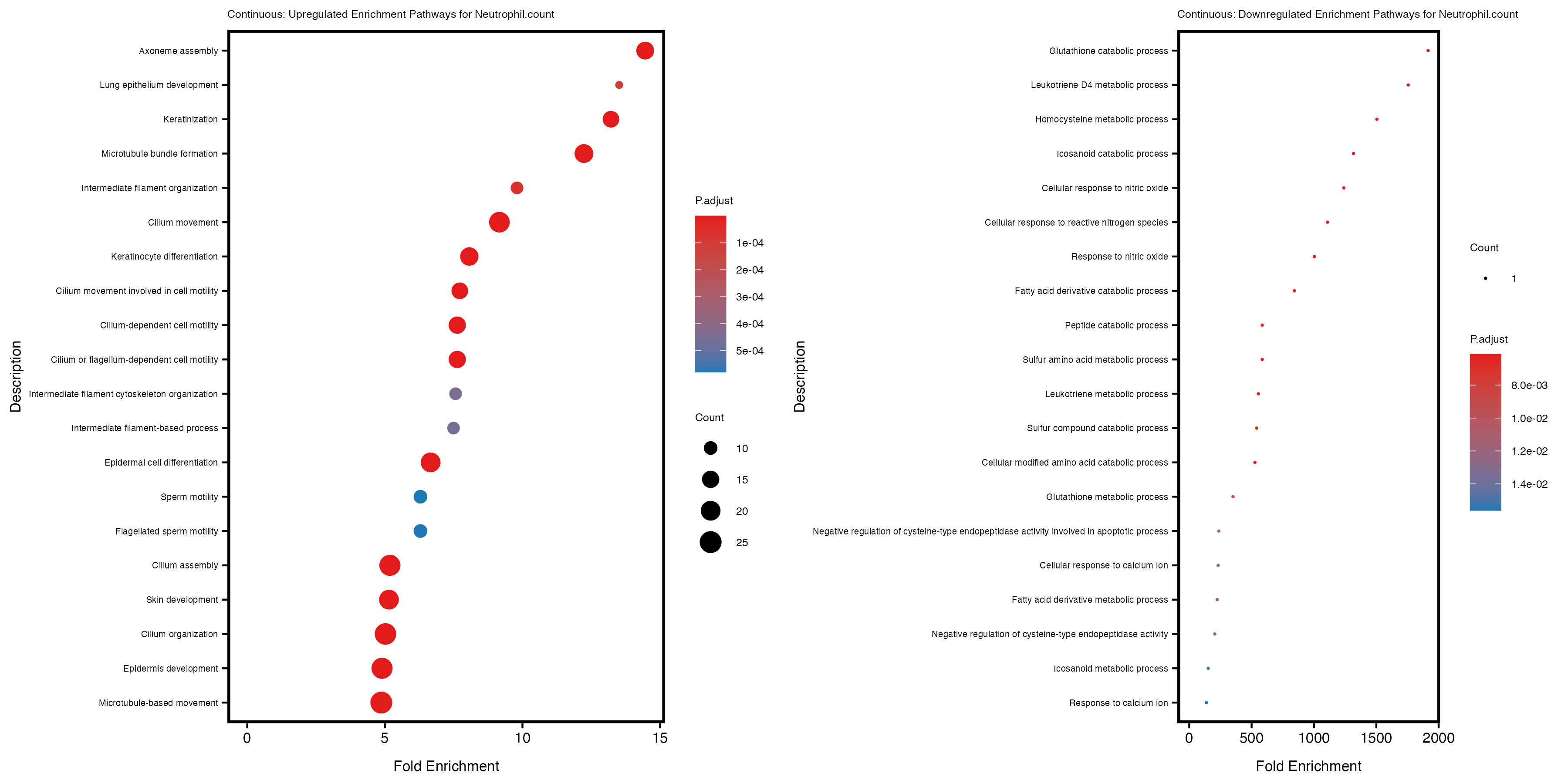
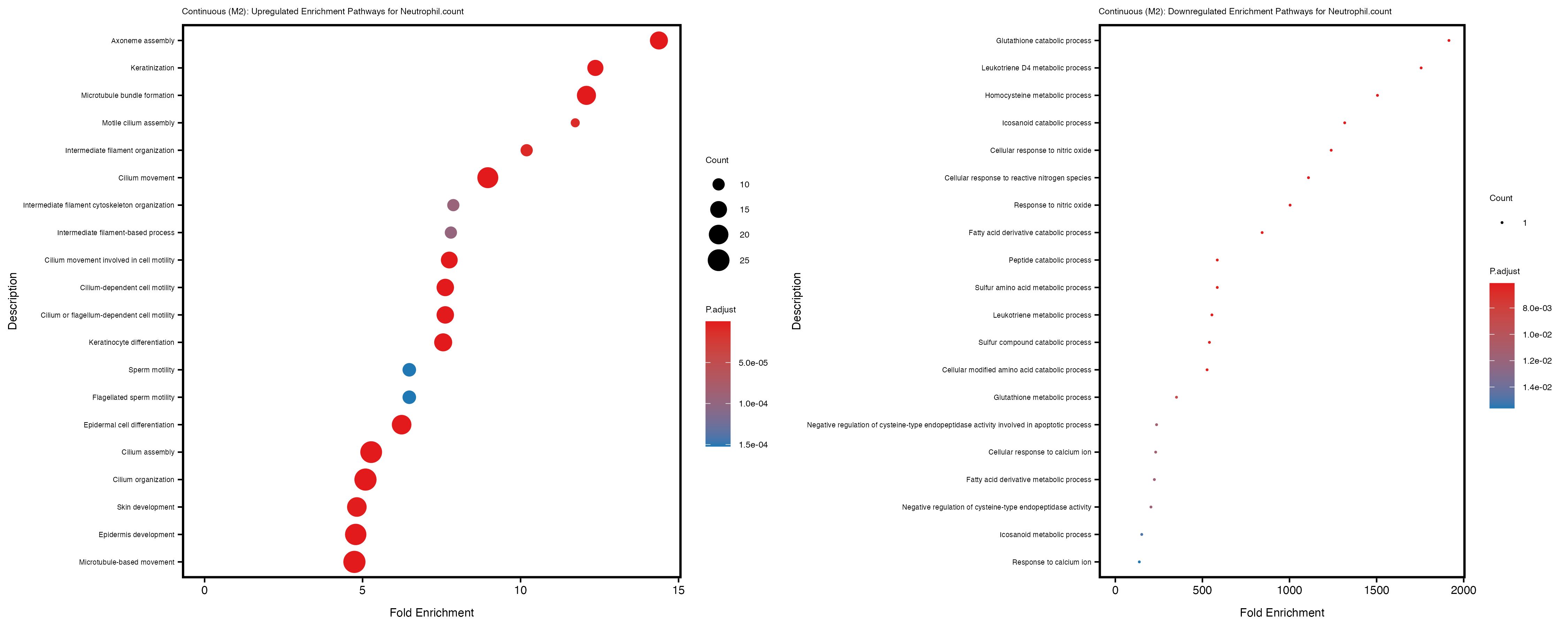
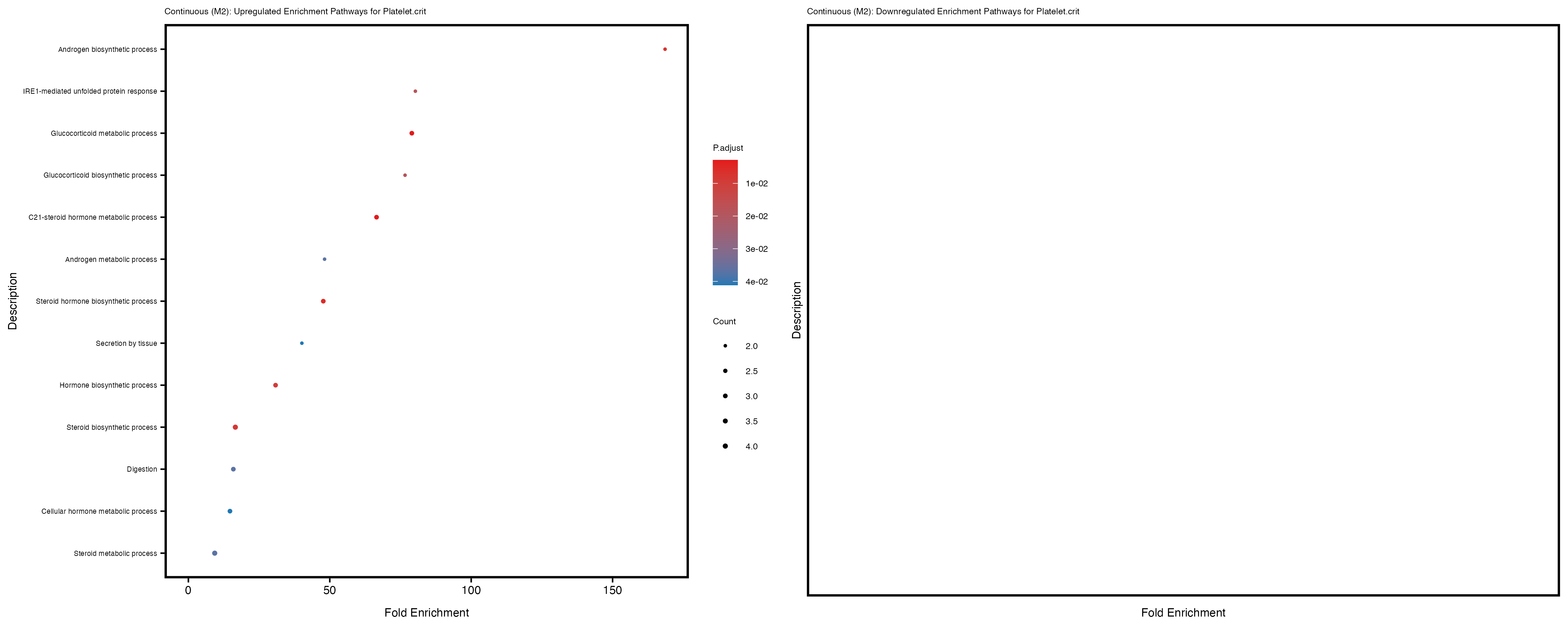
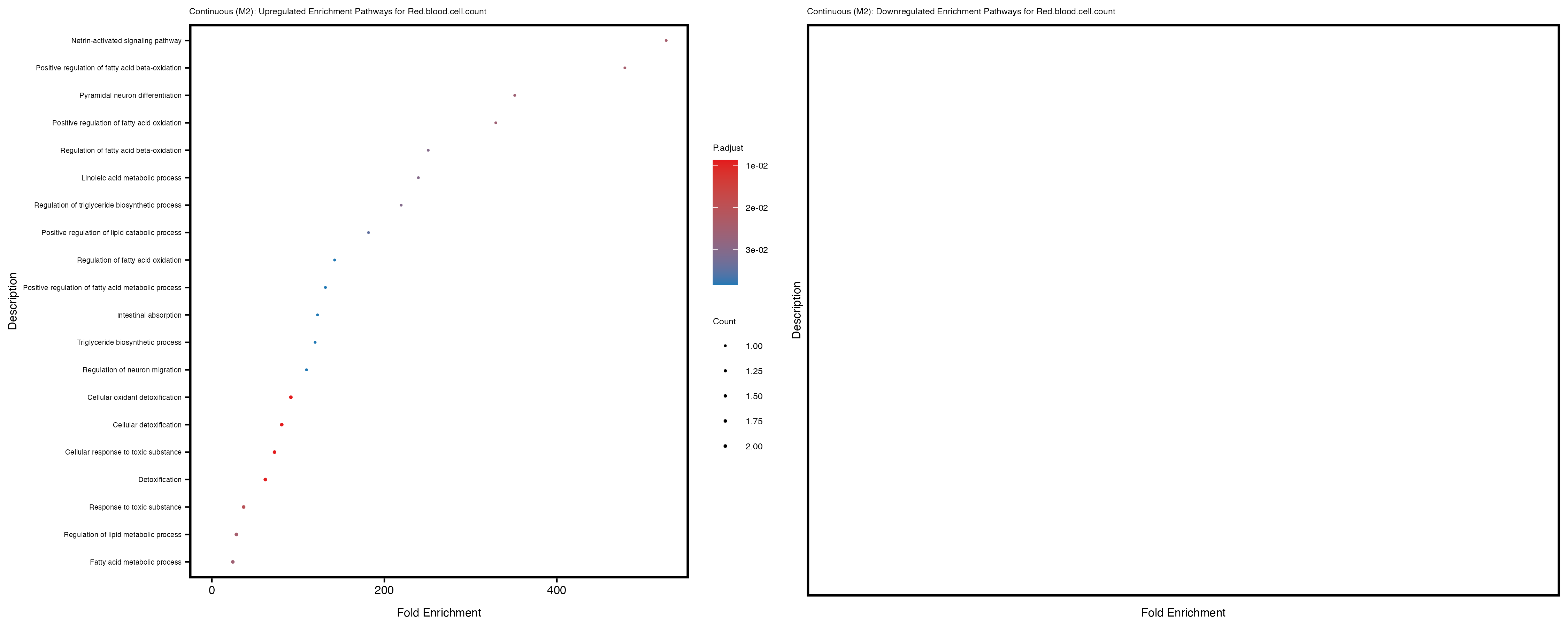
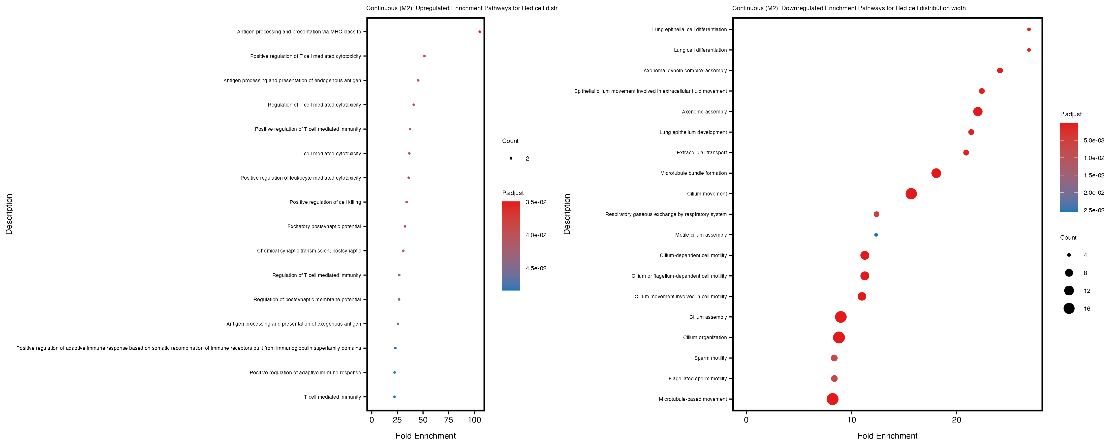
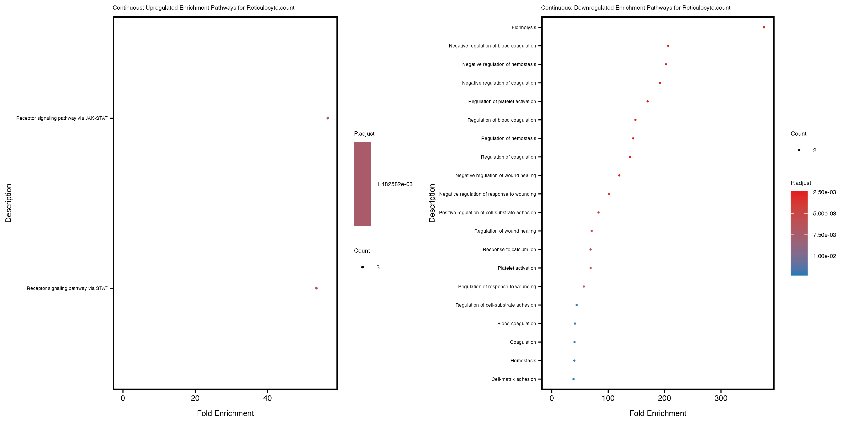
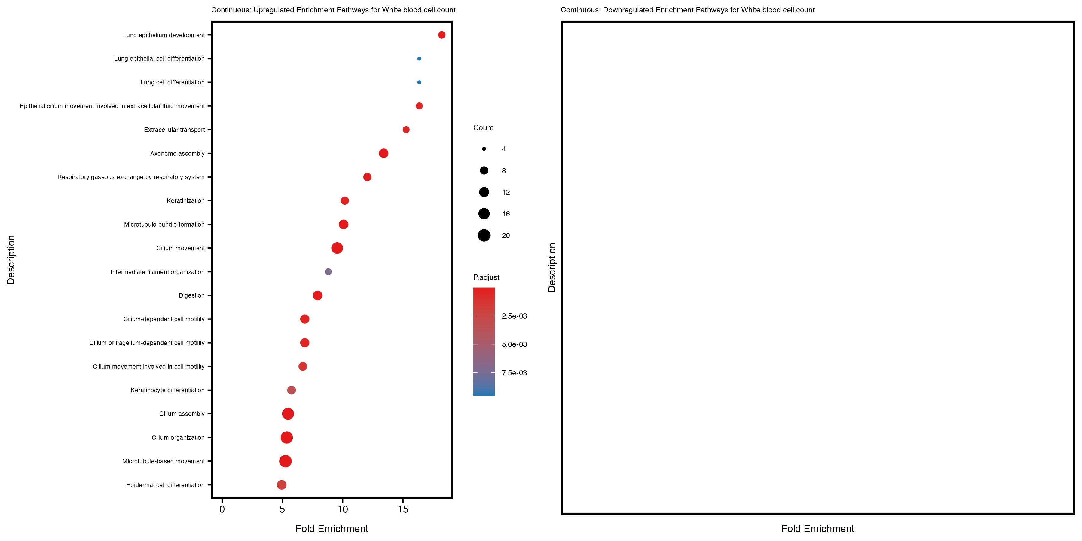
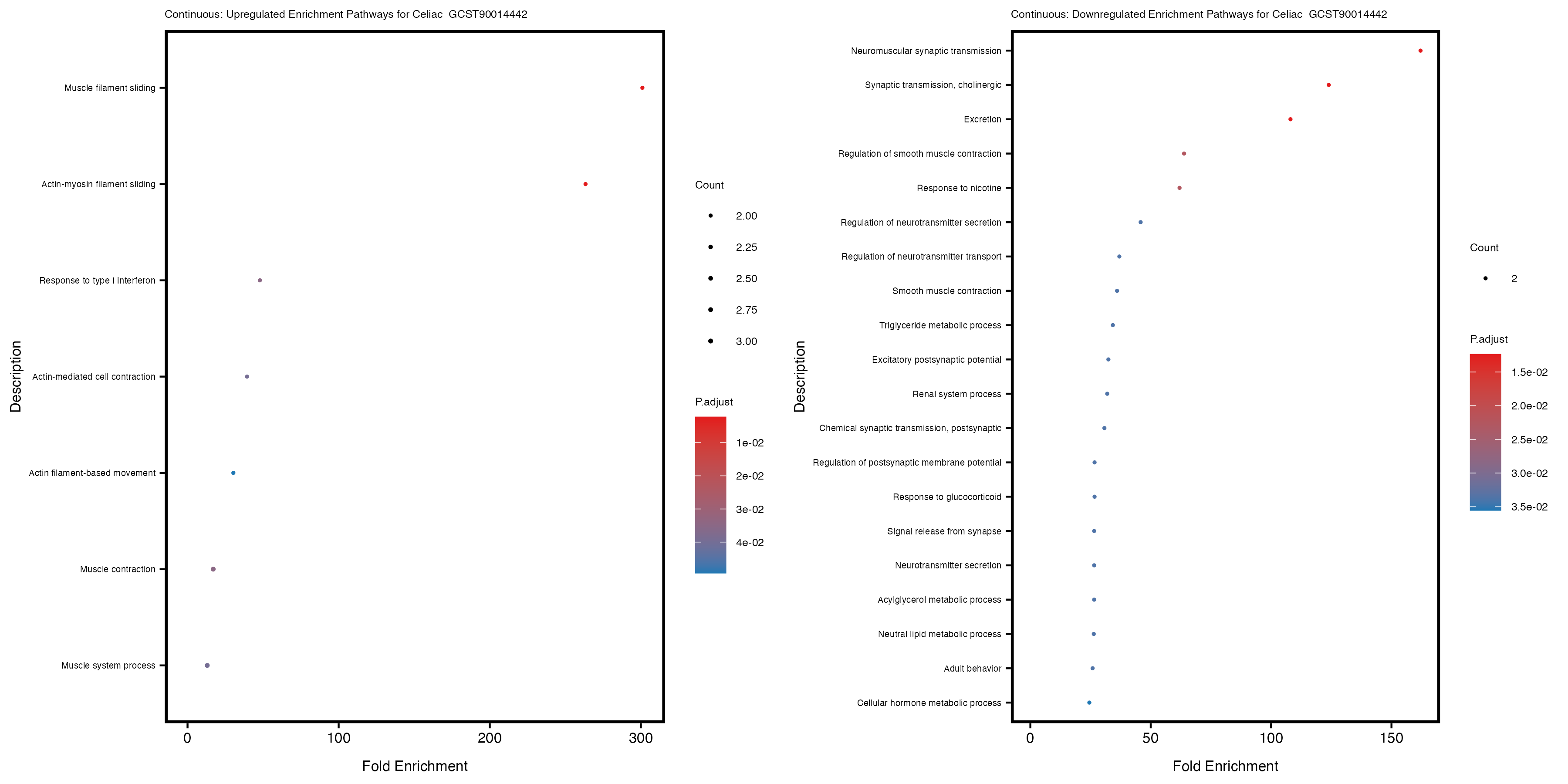
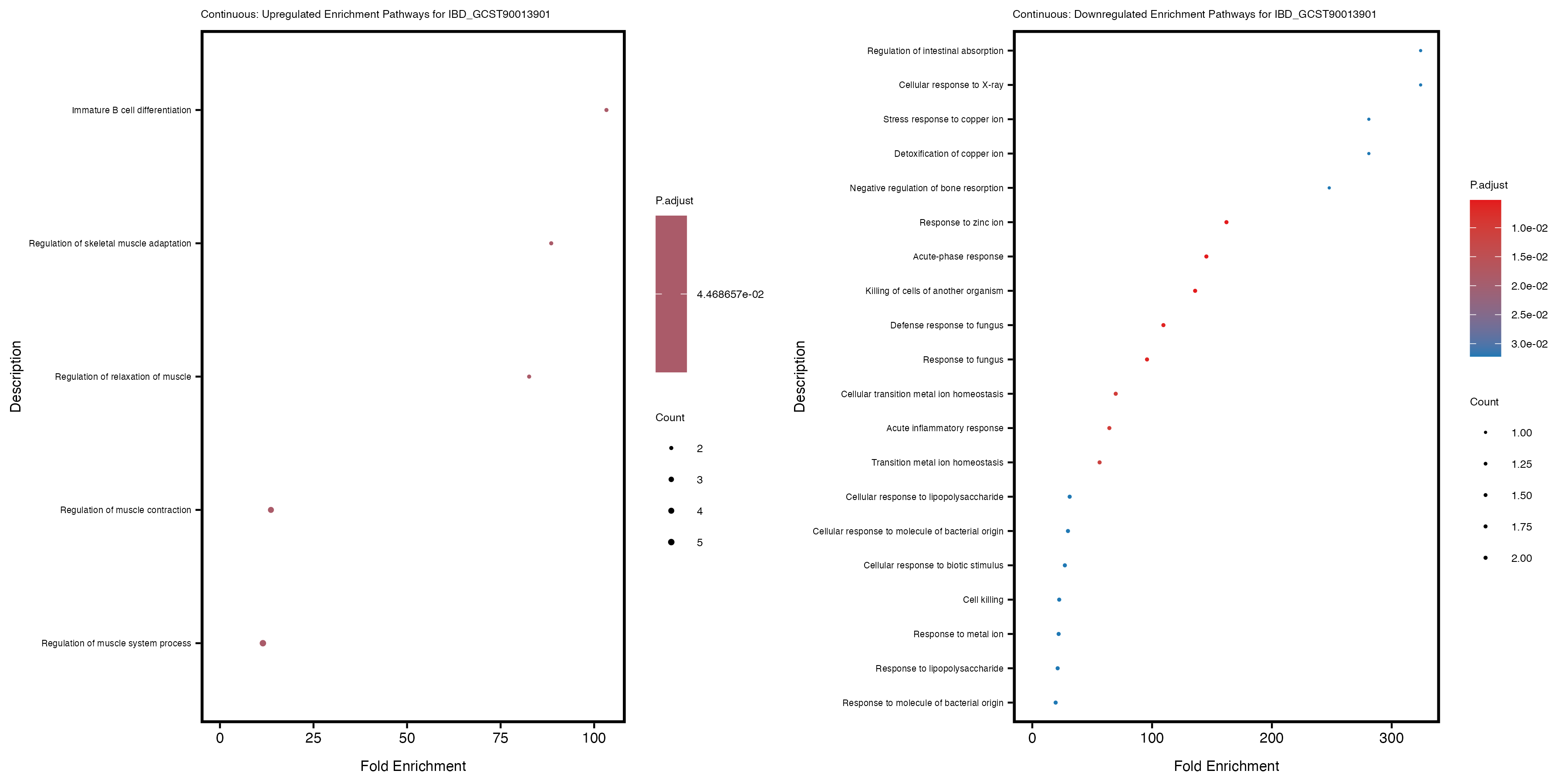
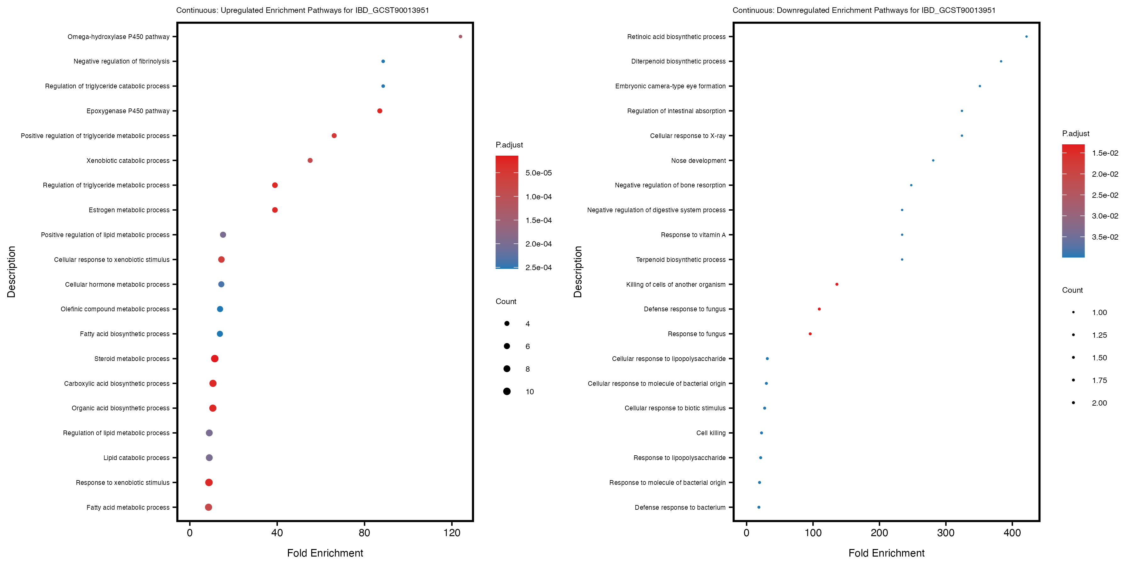
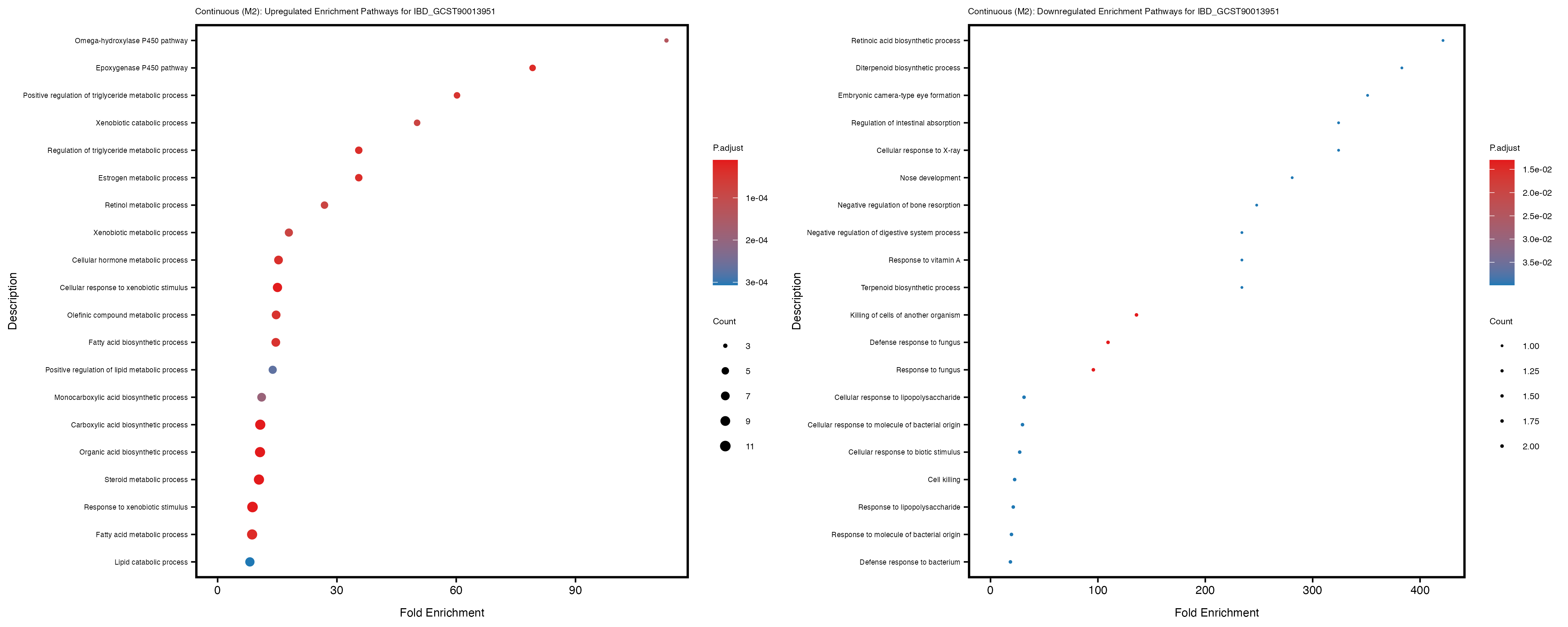
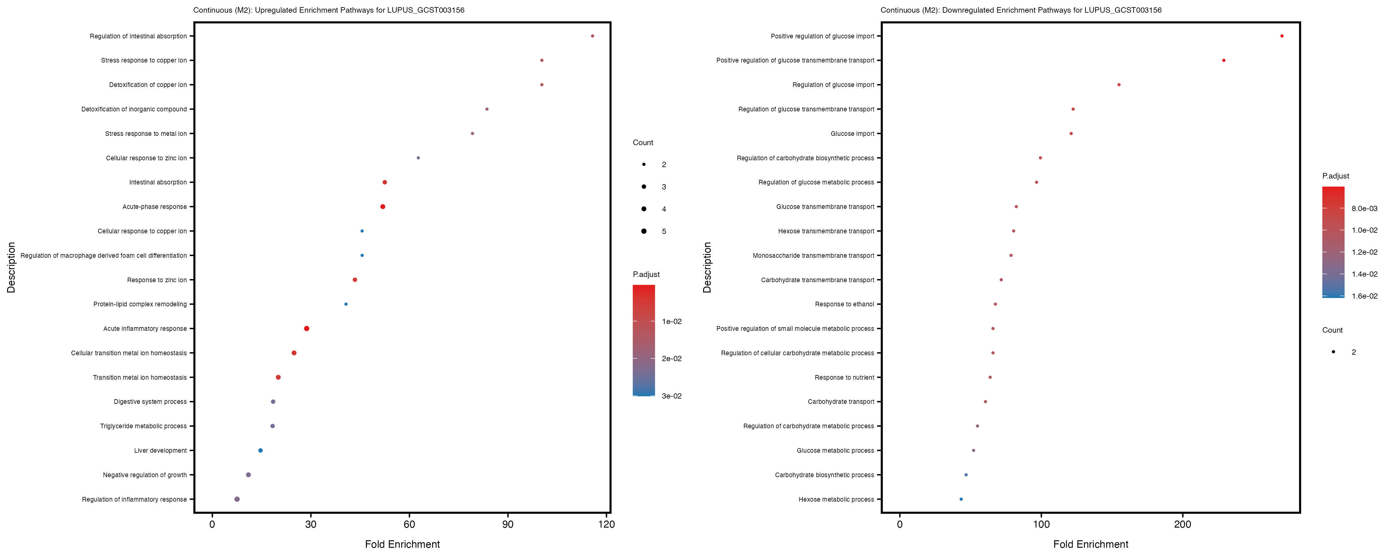
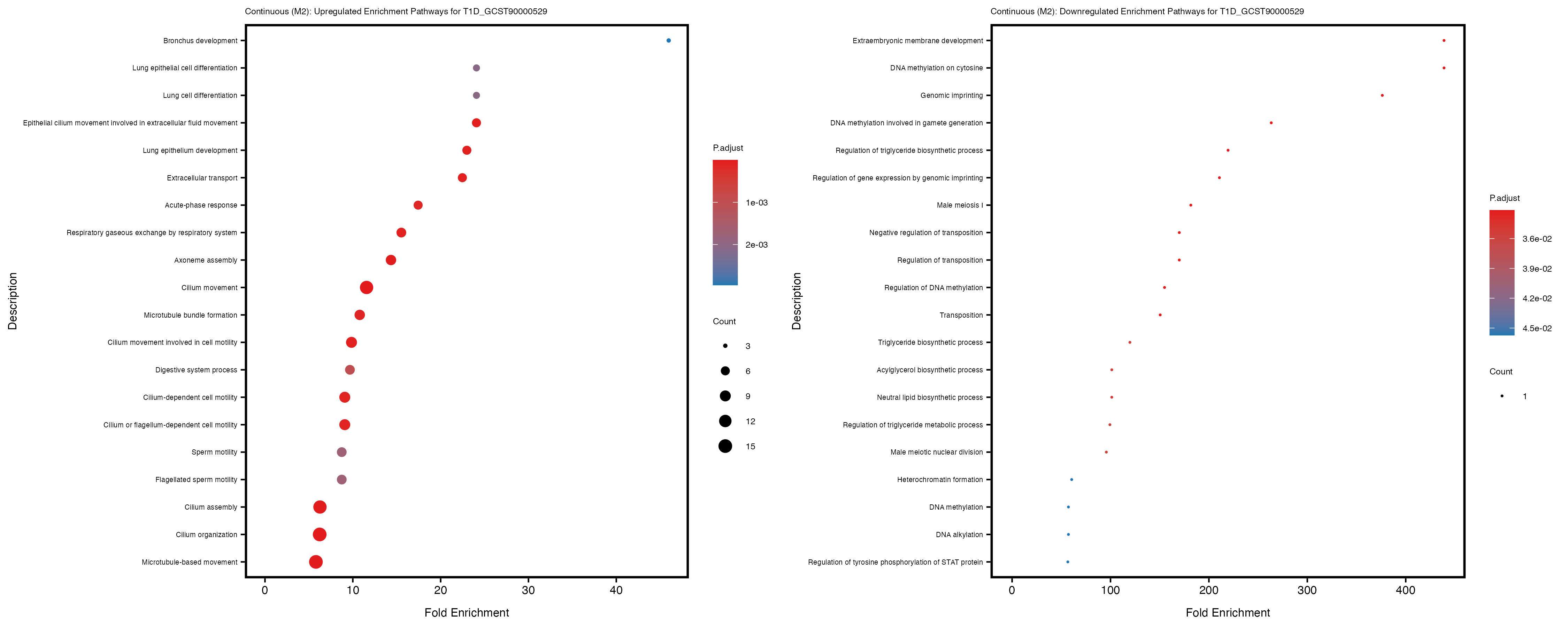
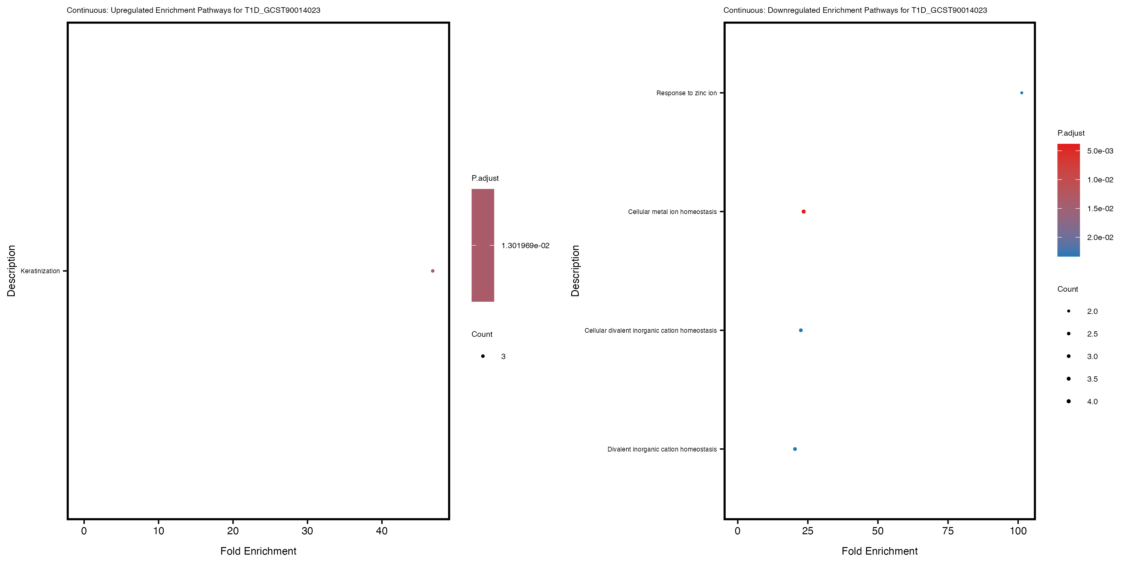
if (nrow(gse_up) >= 20) {
  enrich_plot_up <- plotEnrich(gse_up[1:20, ], plot_type = "dot", scale_ratio = 0.4) +
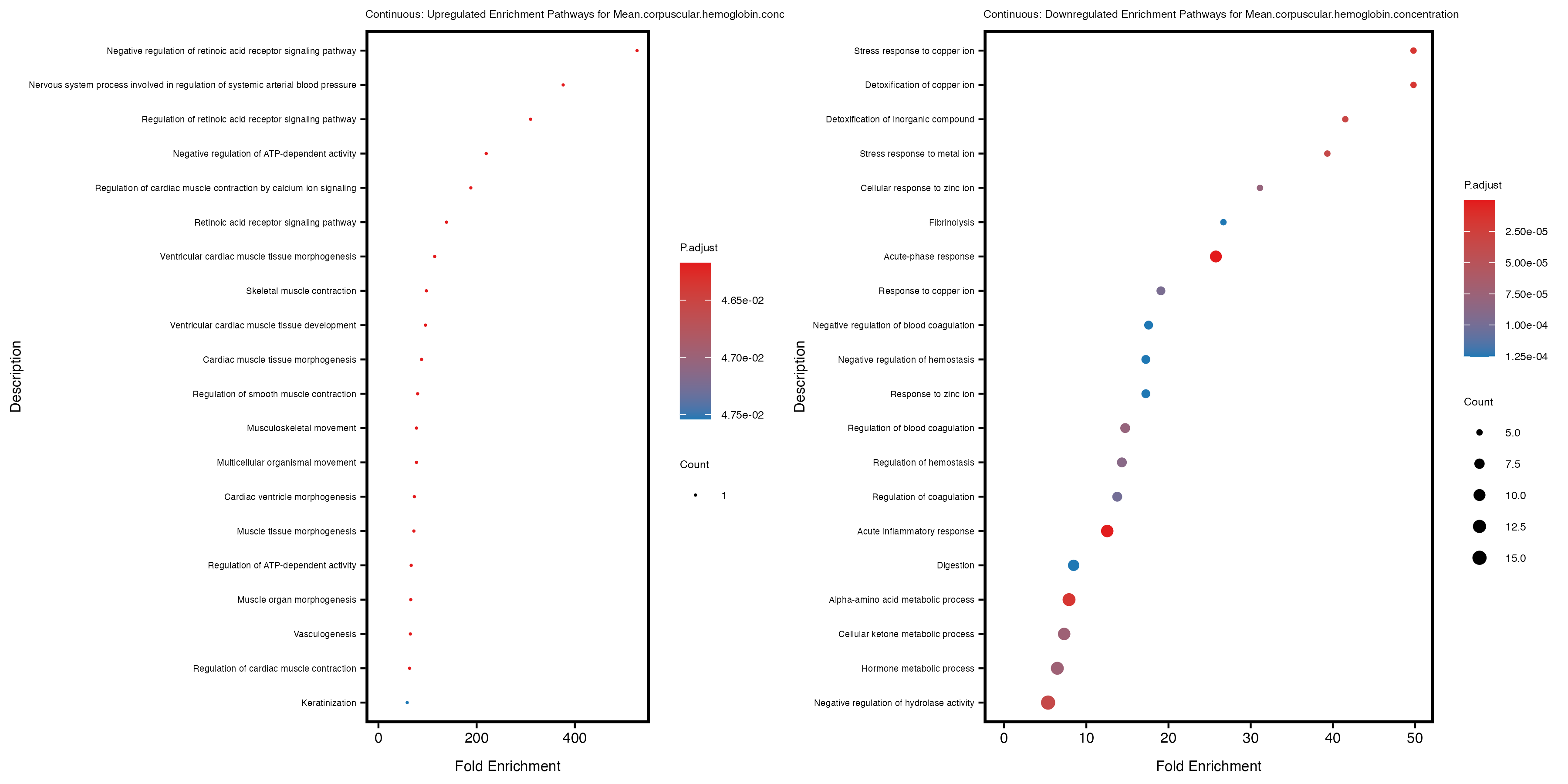
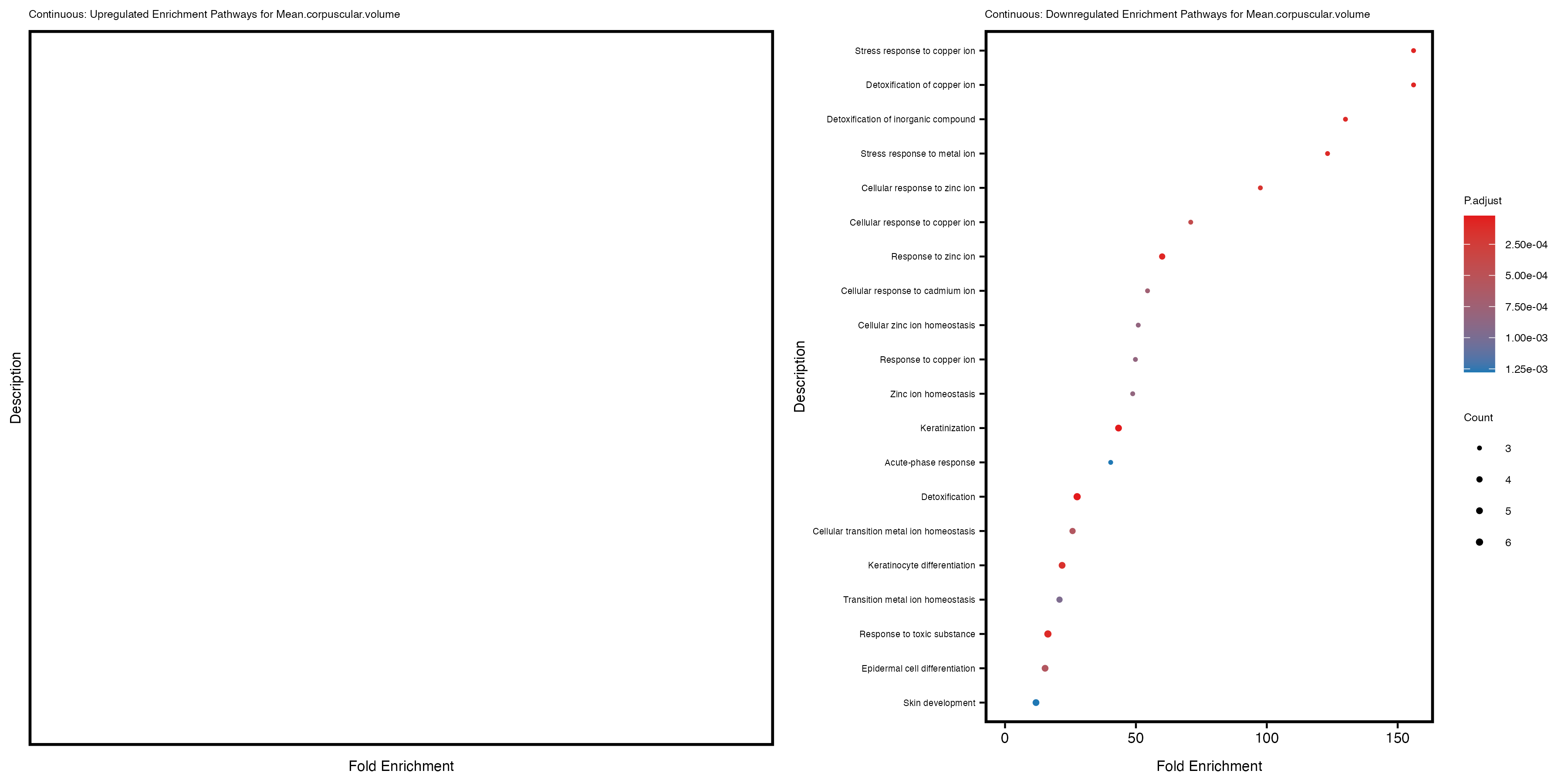
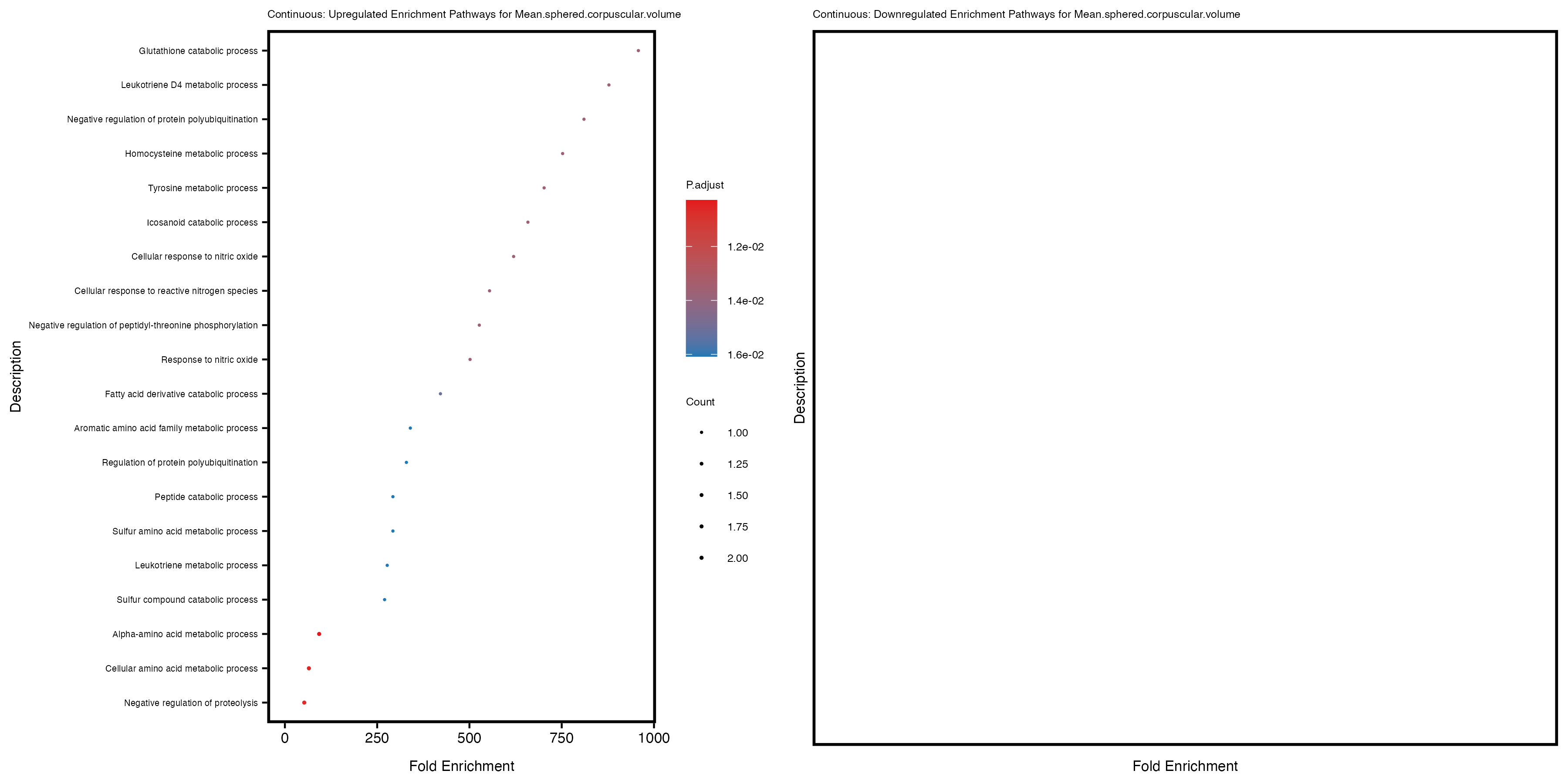
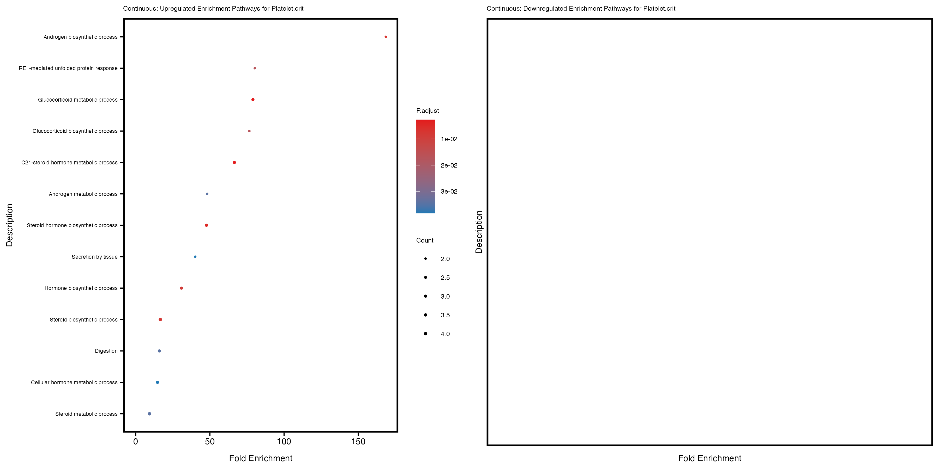
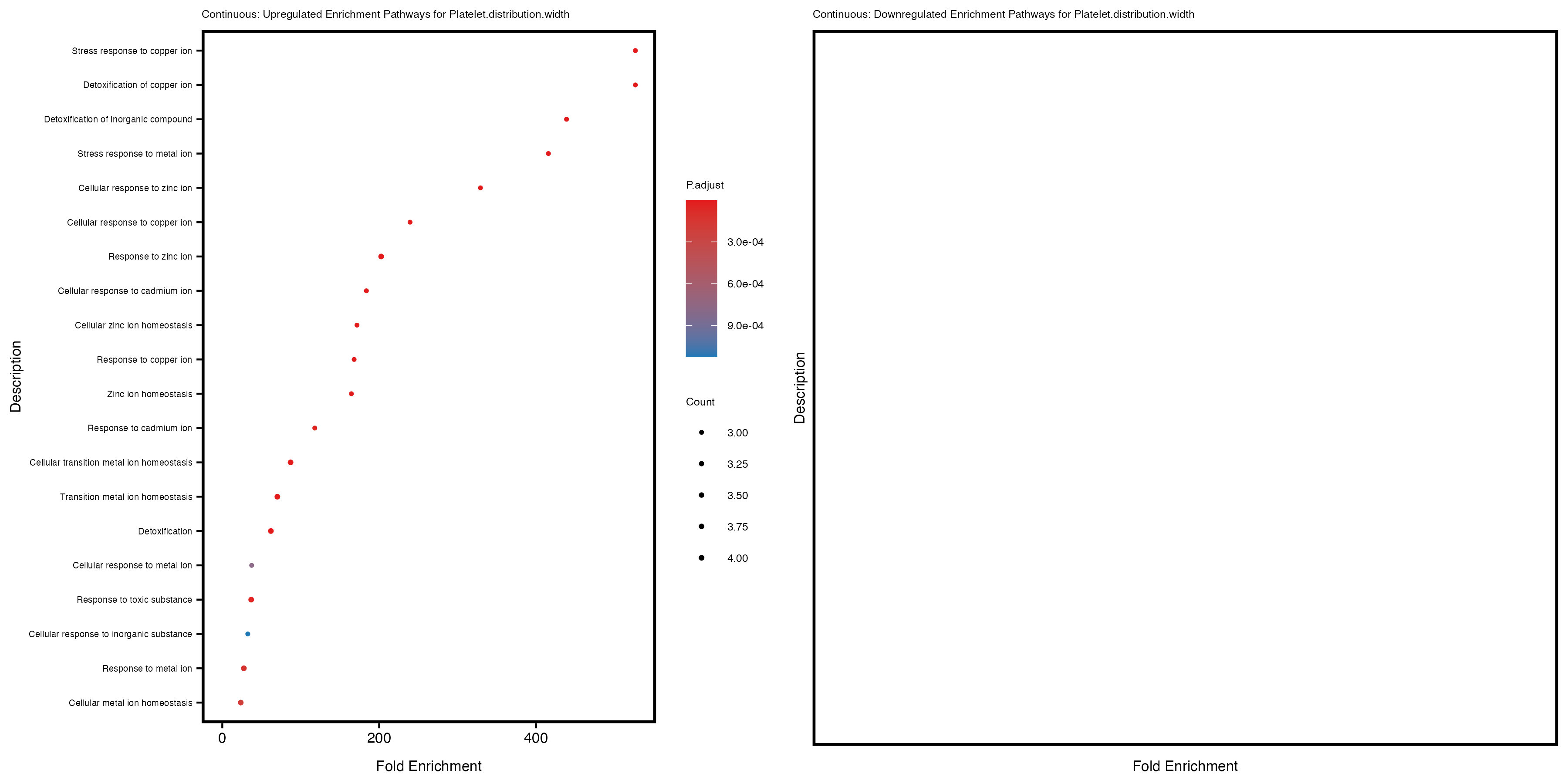
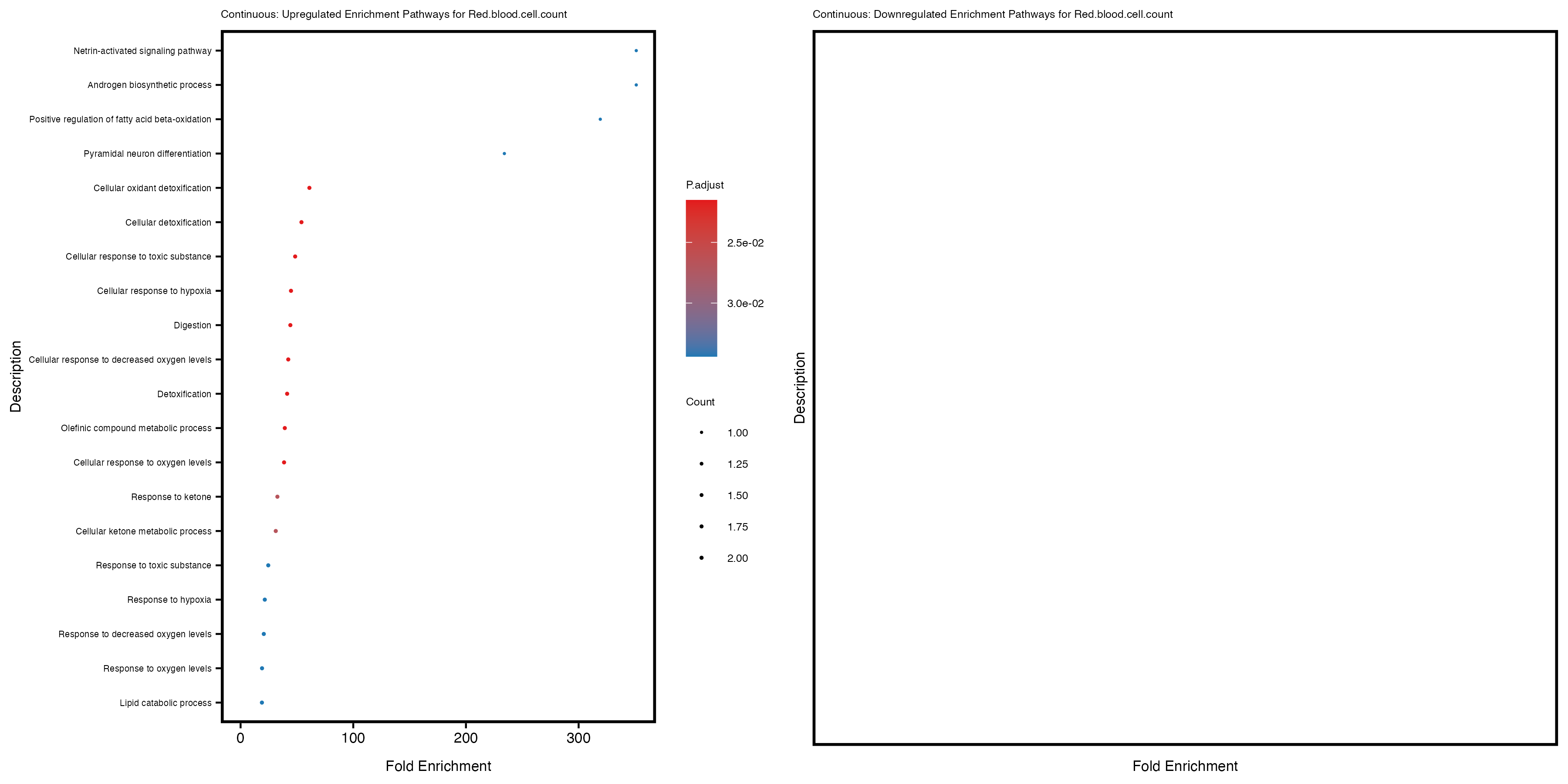
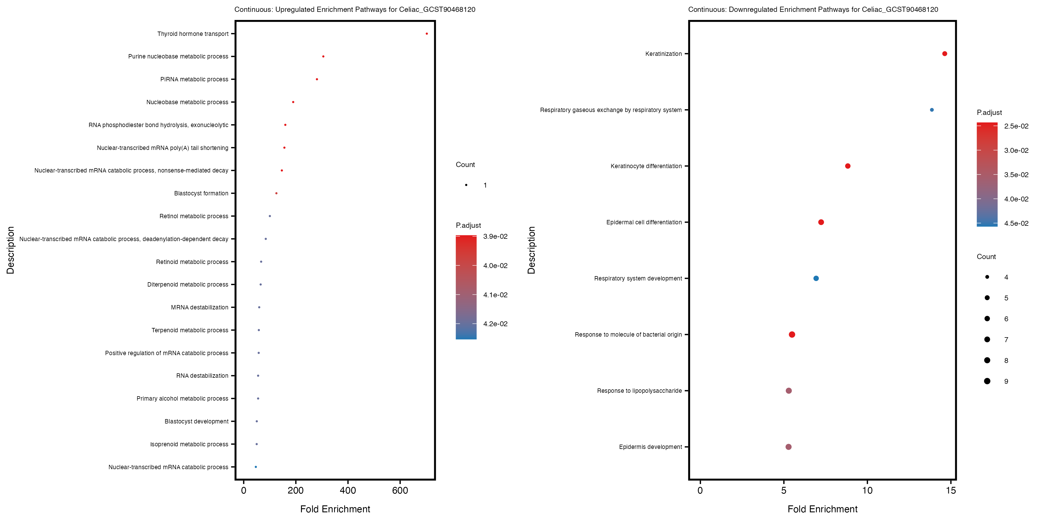
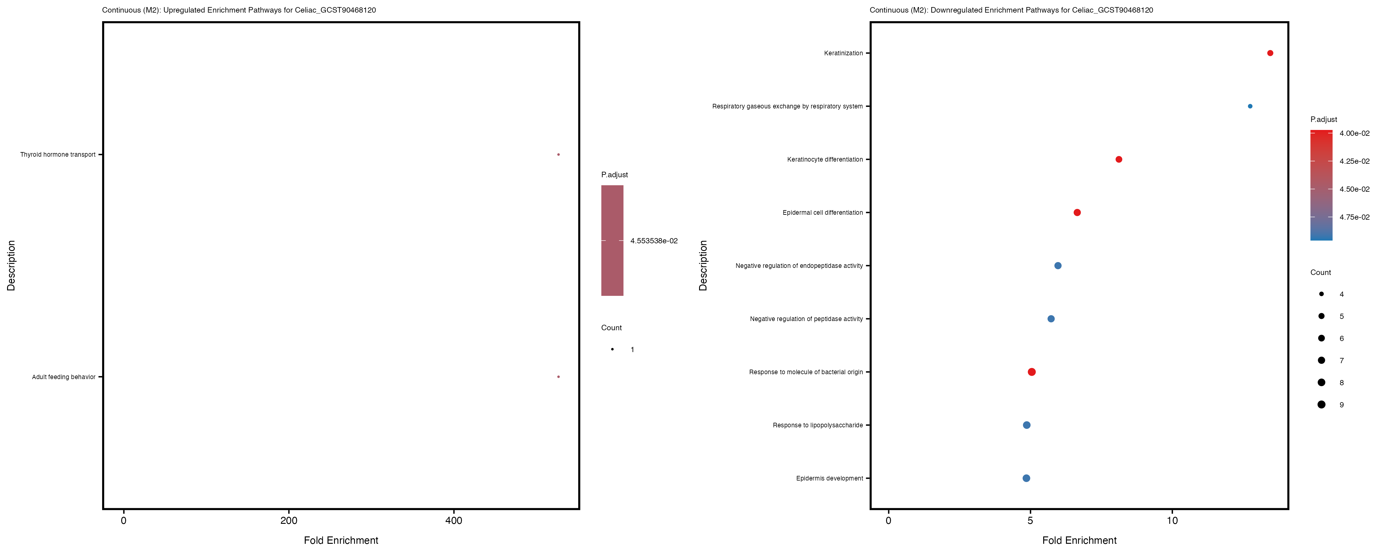
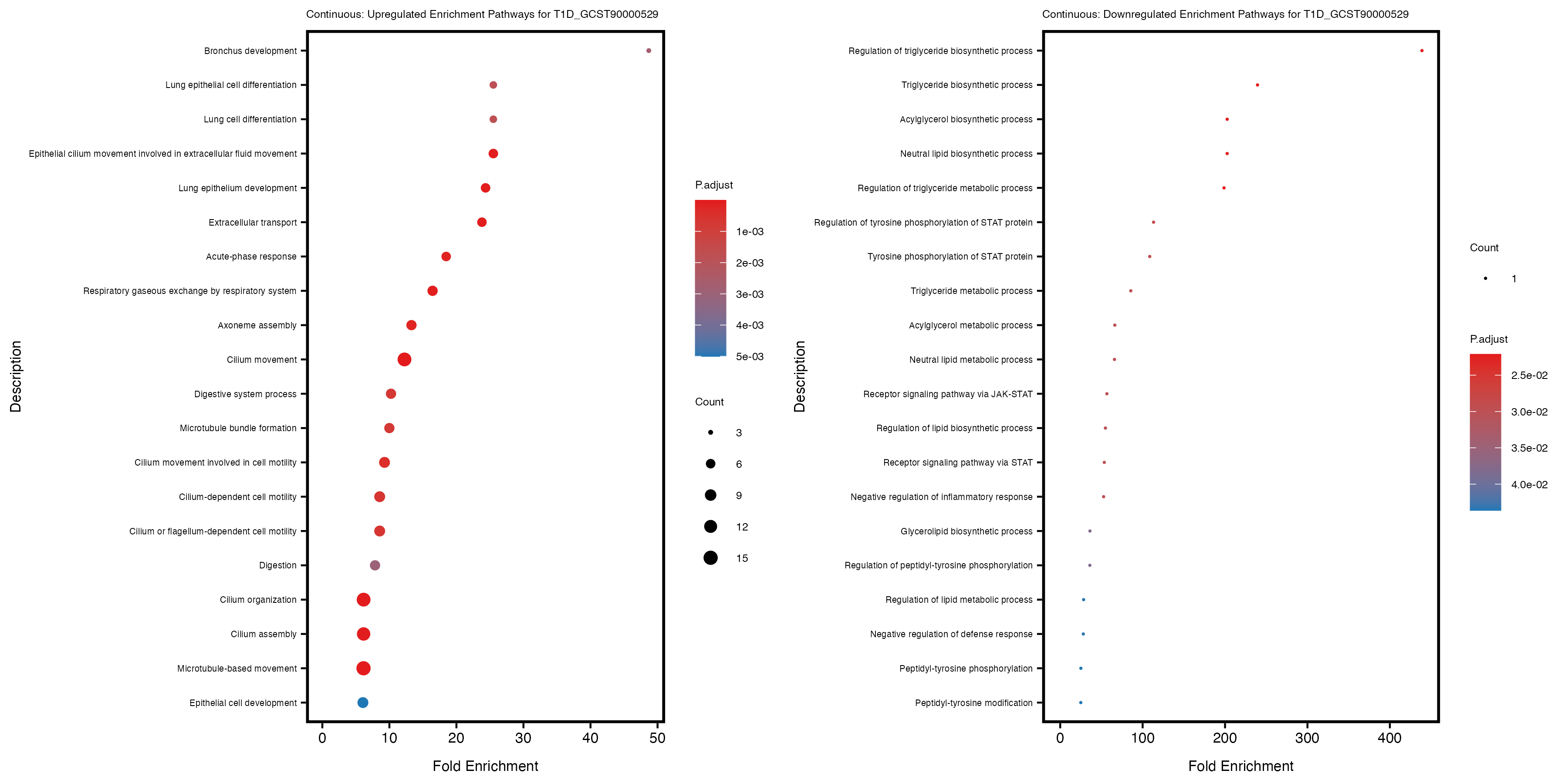
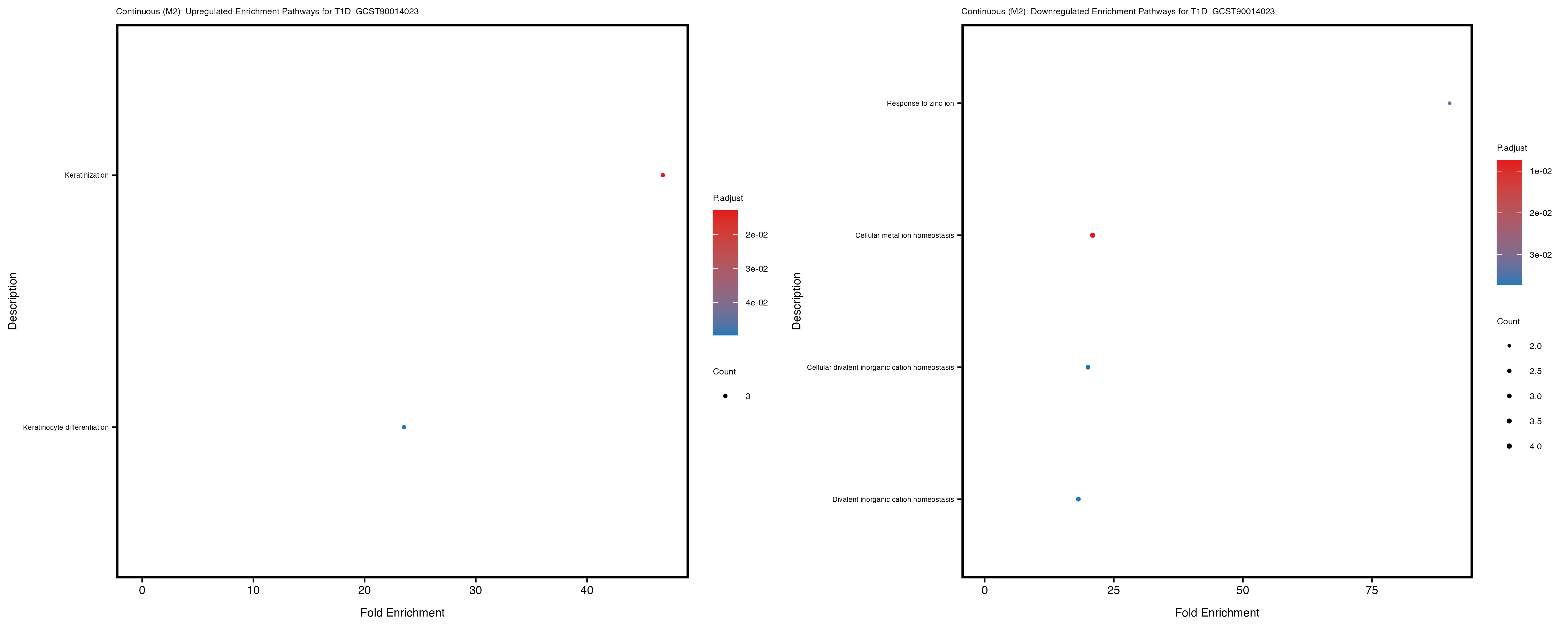
    labs(title = paste("Continuous: Upregulated Enrichment Pathways for", trait)) +
    theme(plot.title = element_text(size = 6), axis.text.y   = element_text(size = 5))
} else {
  enrich_plot_up <- plotEnrich(gse_up, plot_type = "dot", scale_ratio = 0.4) +
    labs(title = paste("Continuous: Upregulated Enrichment Pathways for", trait)) +
    theme(plot.title = element_text(size = 6), axis.text.y   = element_text(size = 5))
}
  
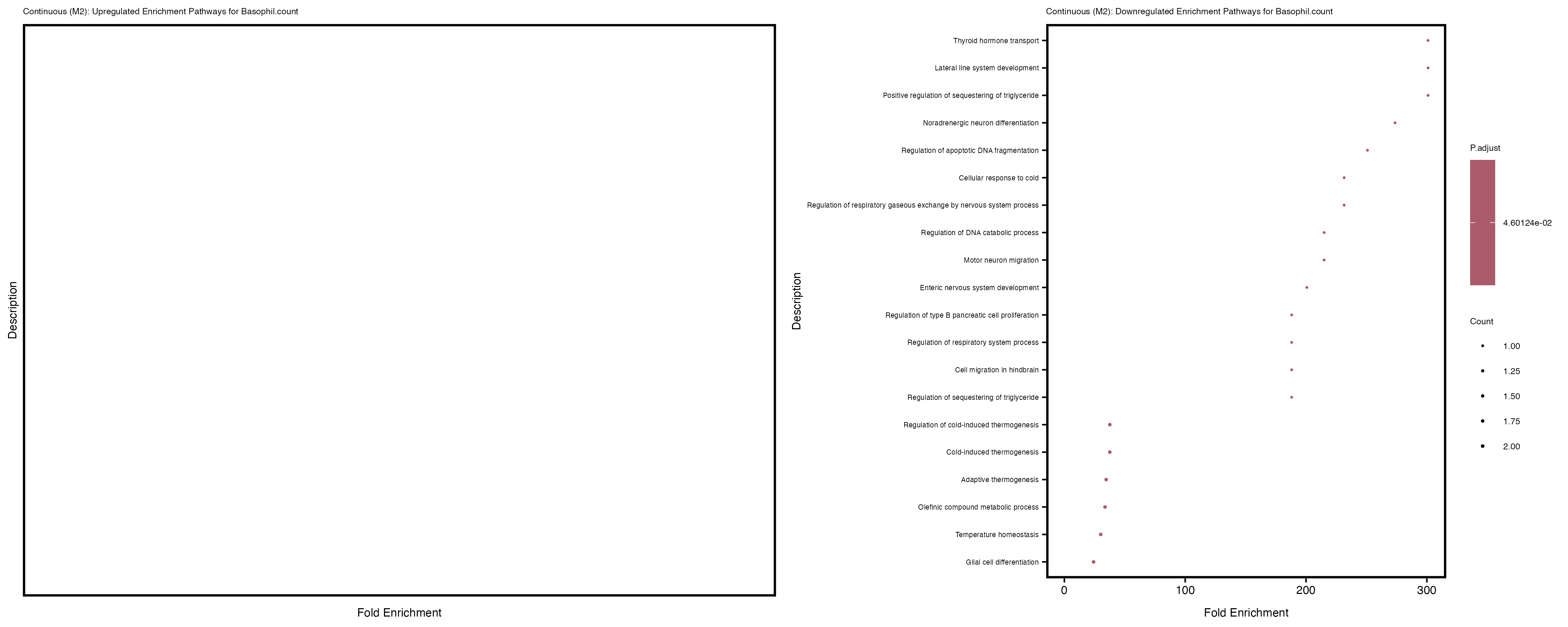
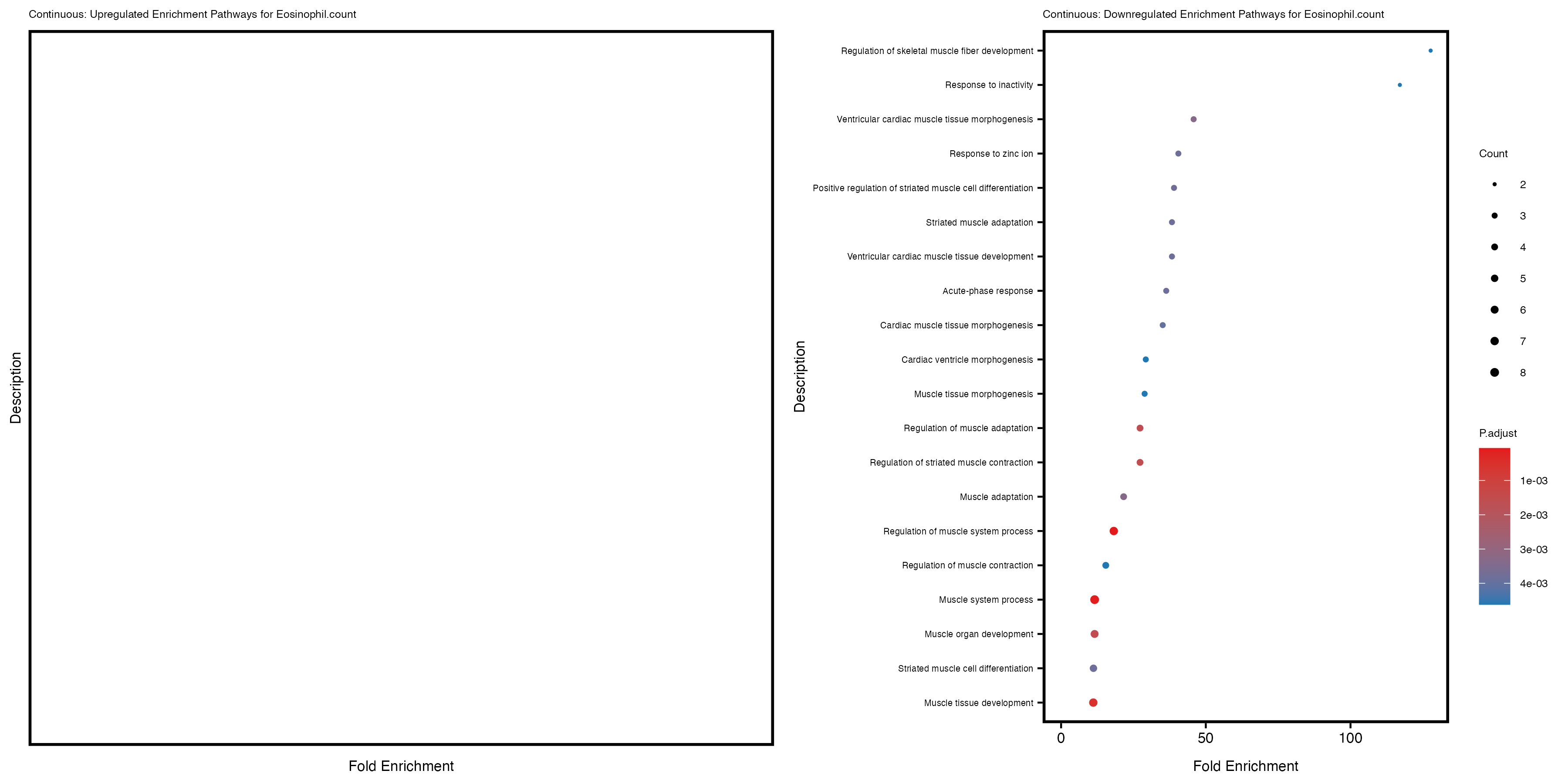
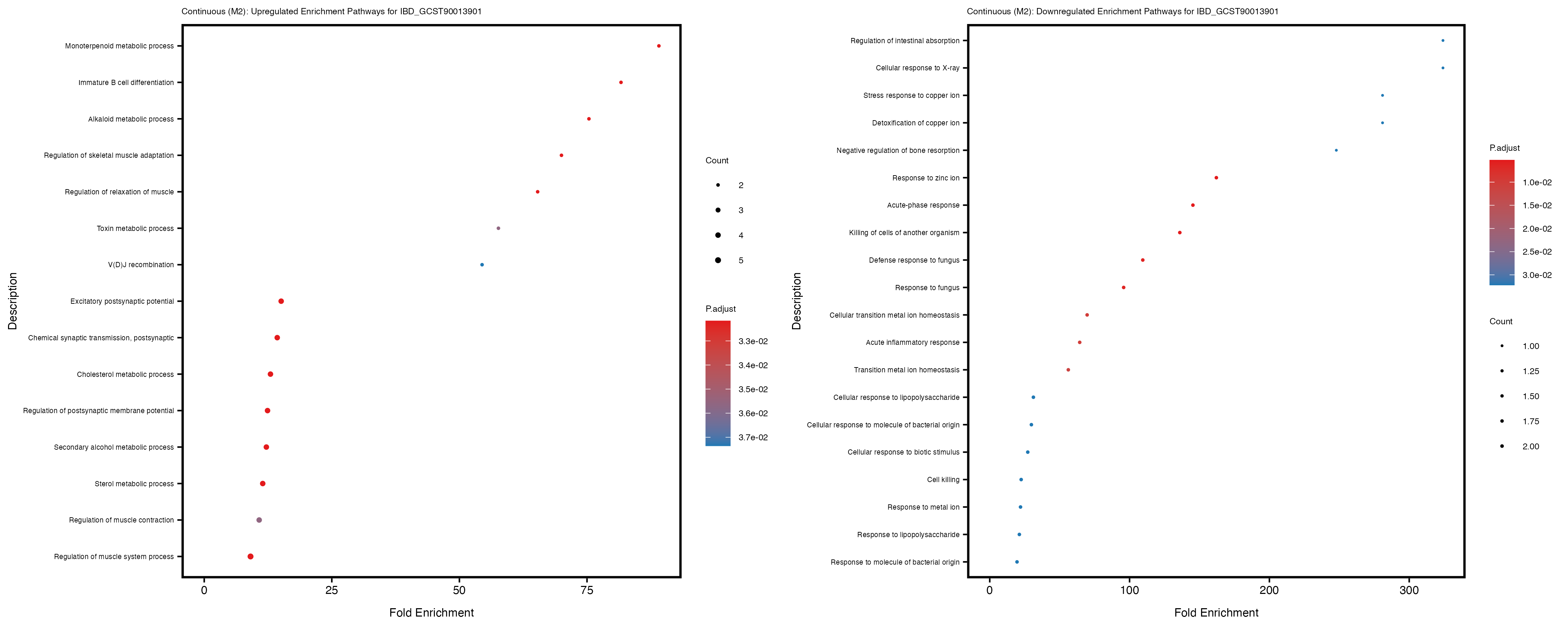
if (nrow(gse_down) >= 20) {
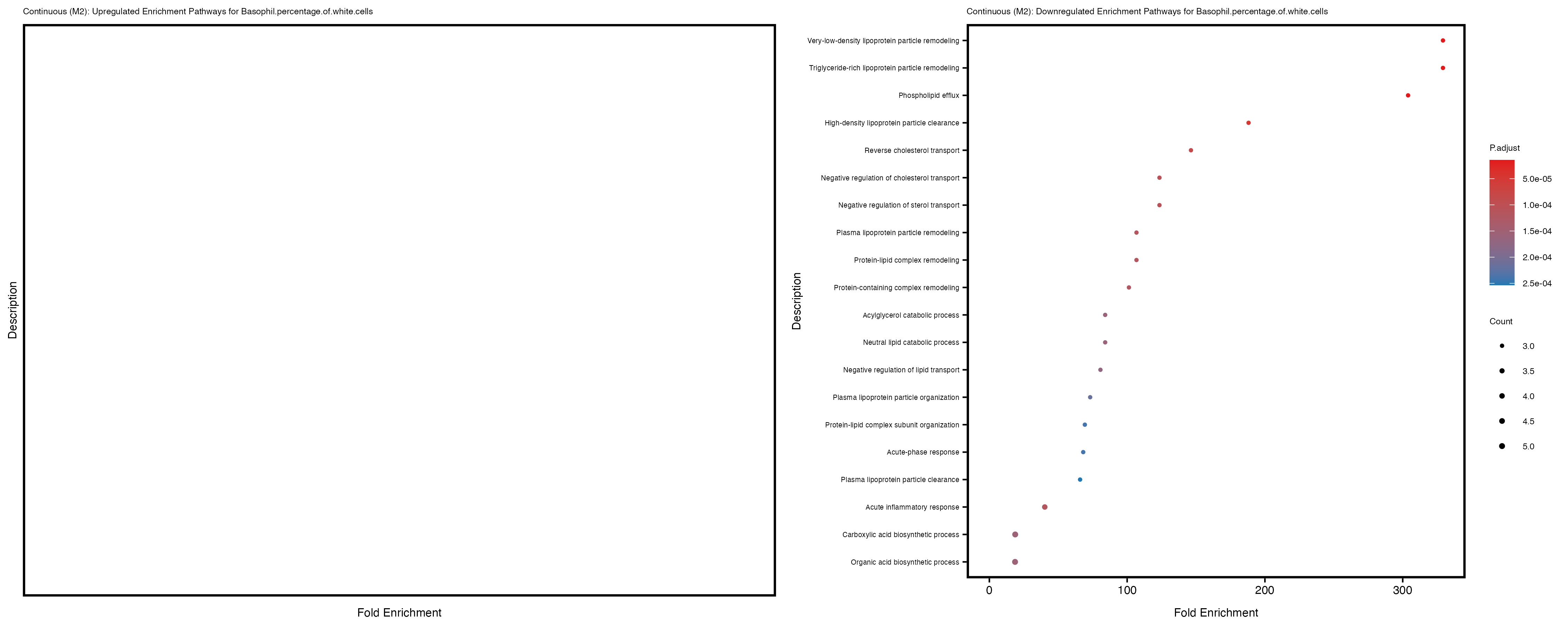
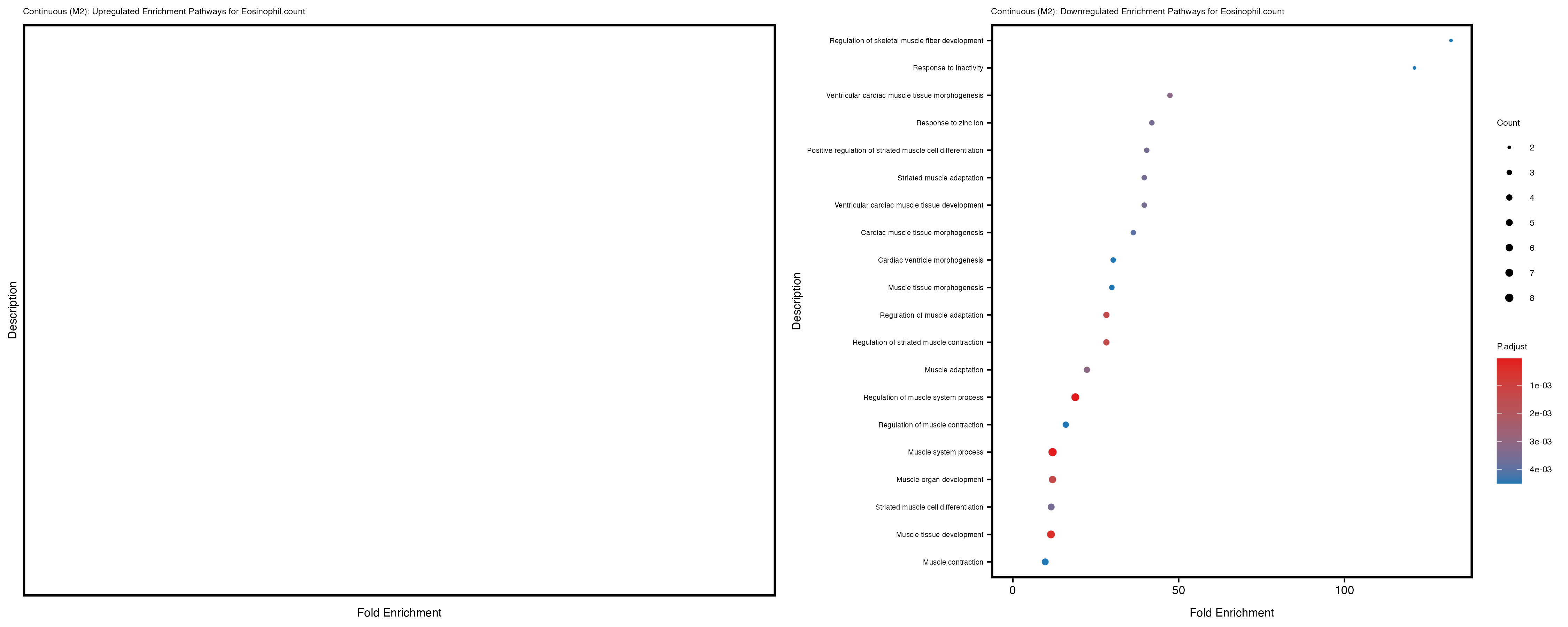
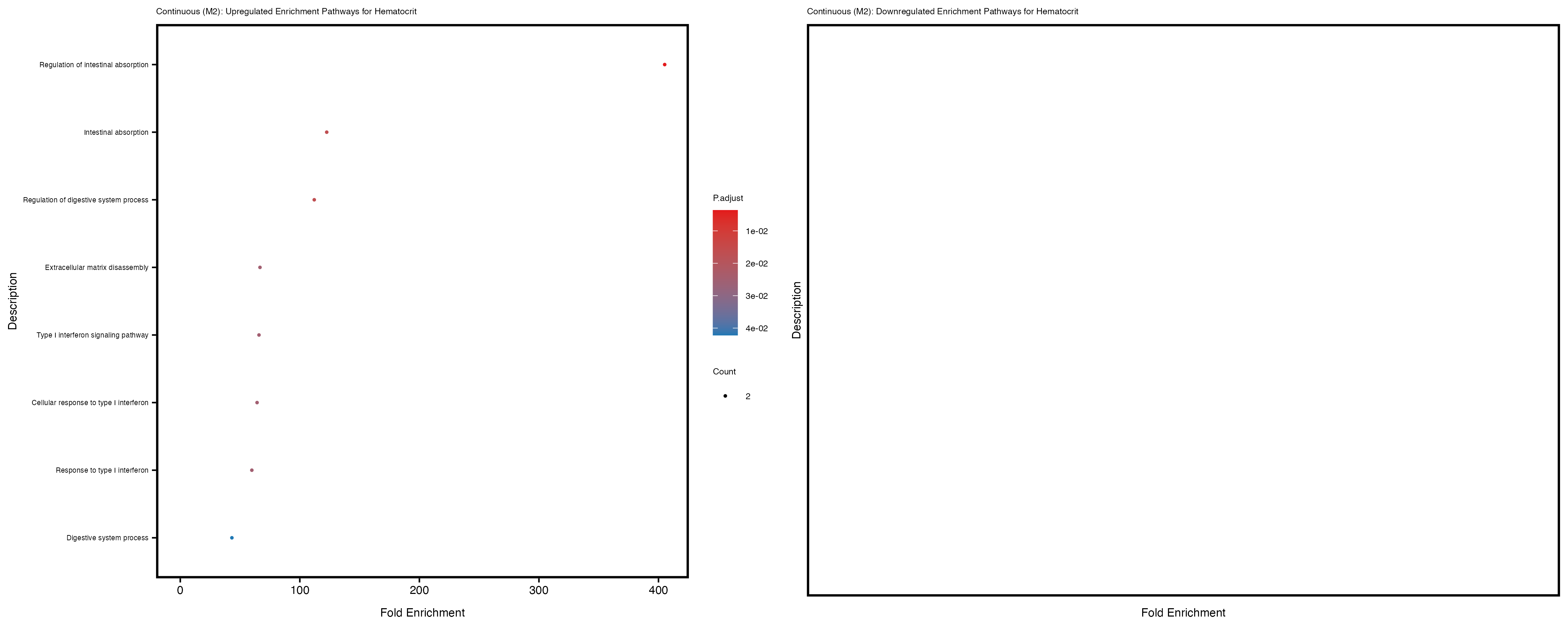
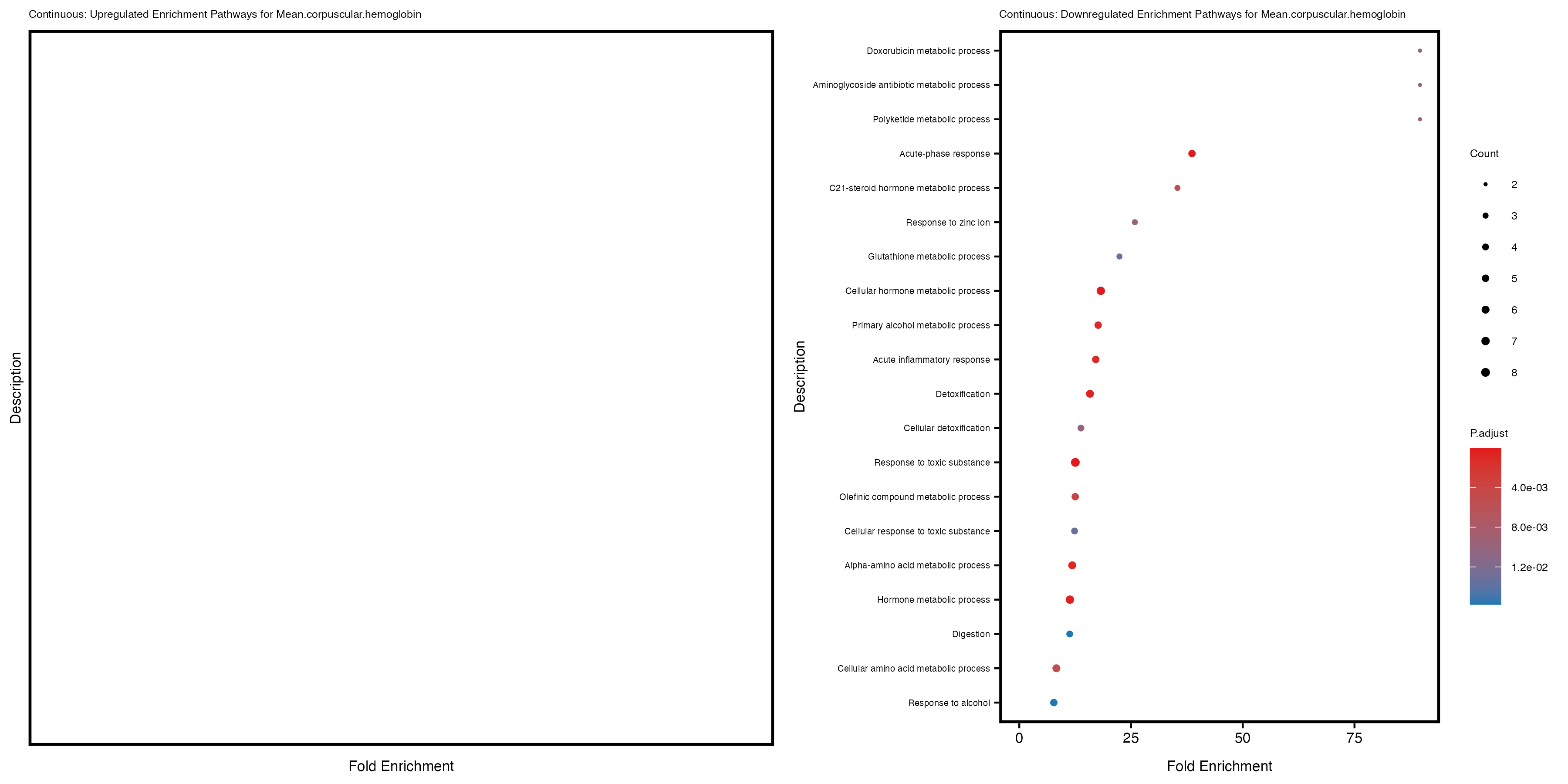
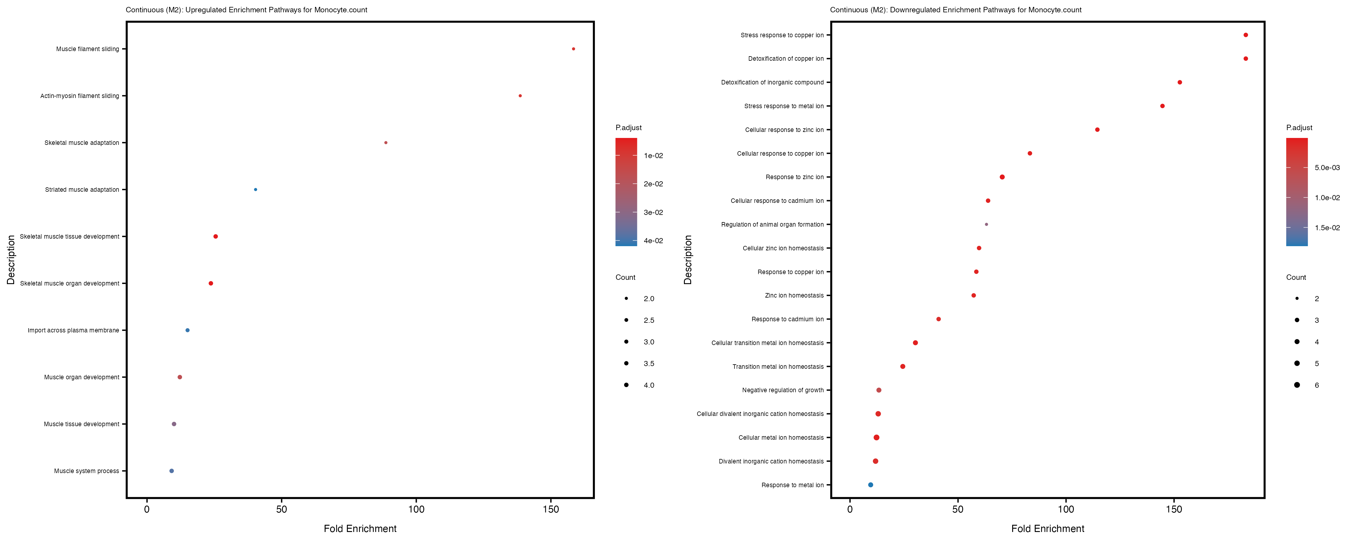
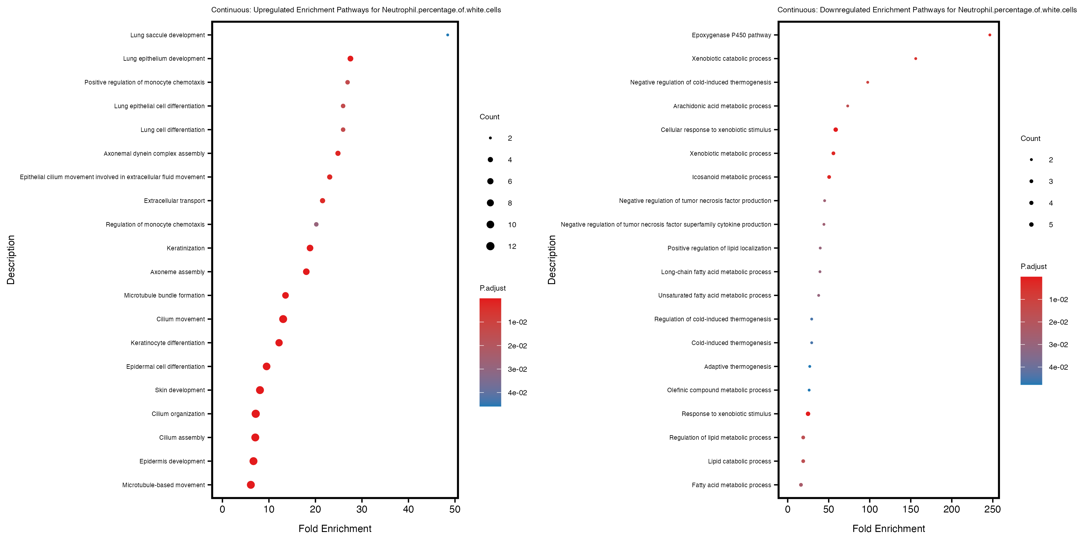
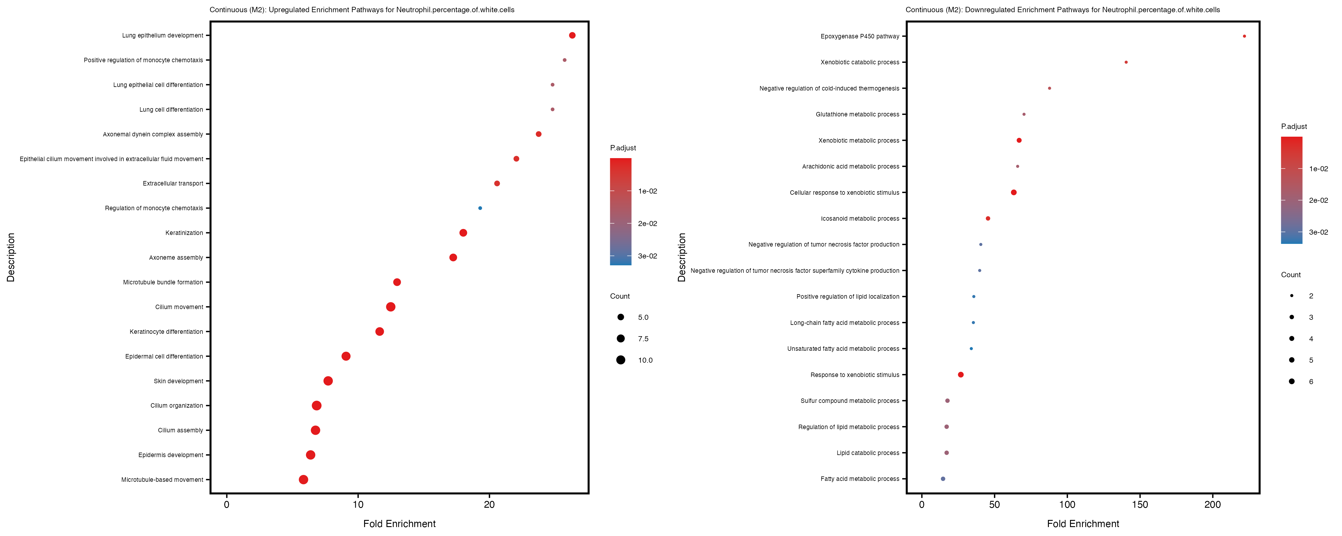
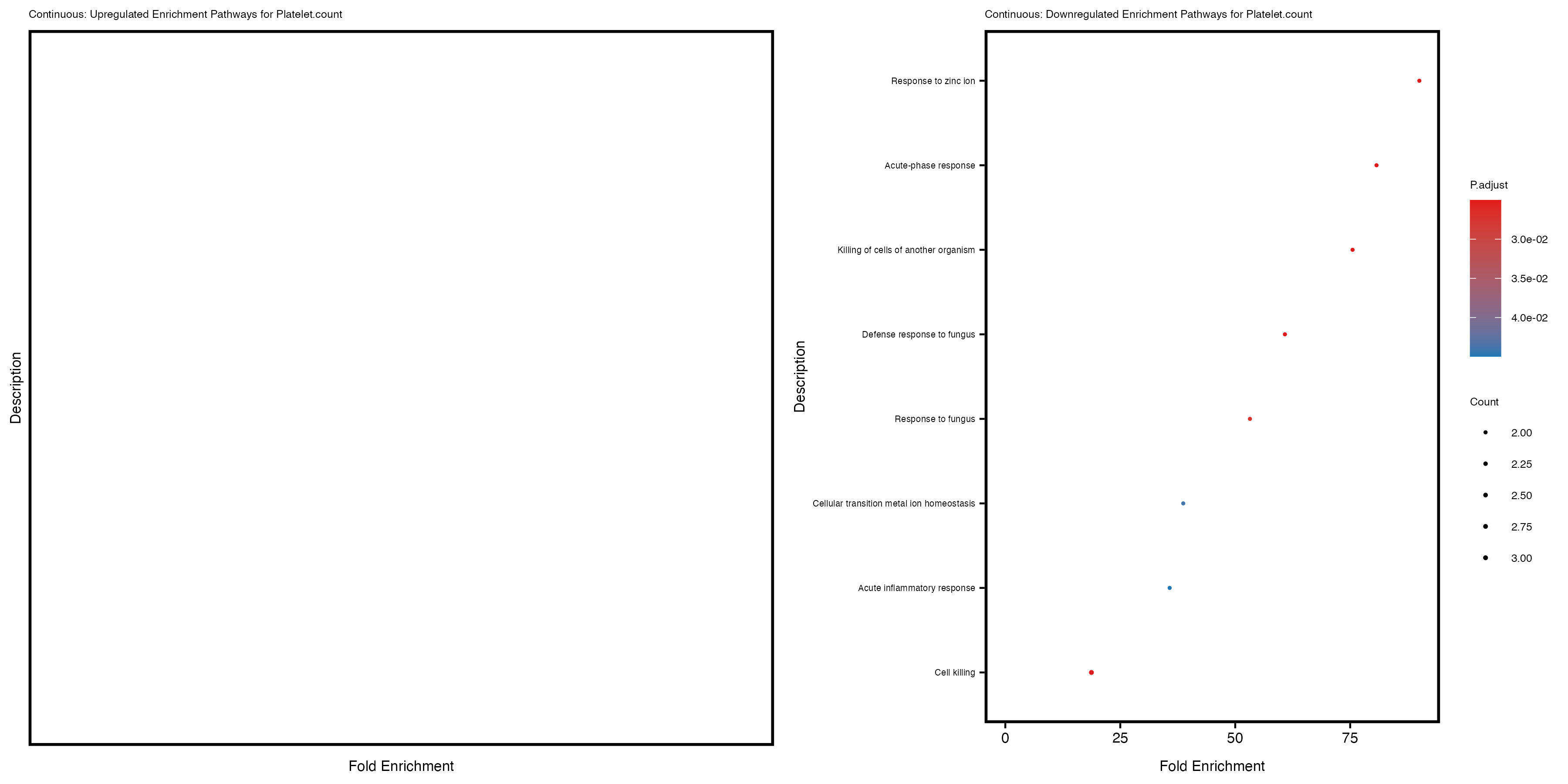
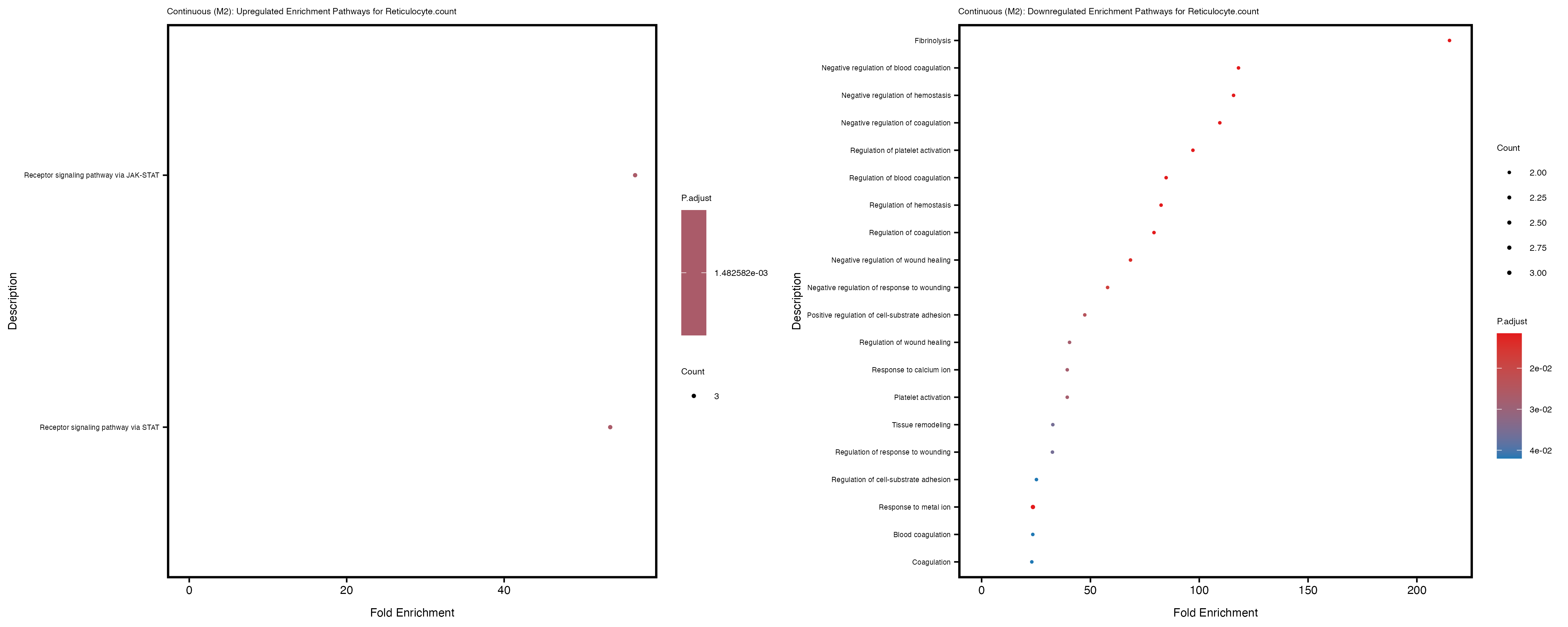
  enrich_plot_down <- plotEnrich(gse_down[1:20, ], plot_type = "dot", scale_ratio = 0.4) +
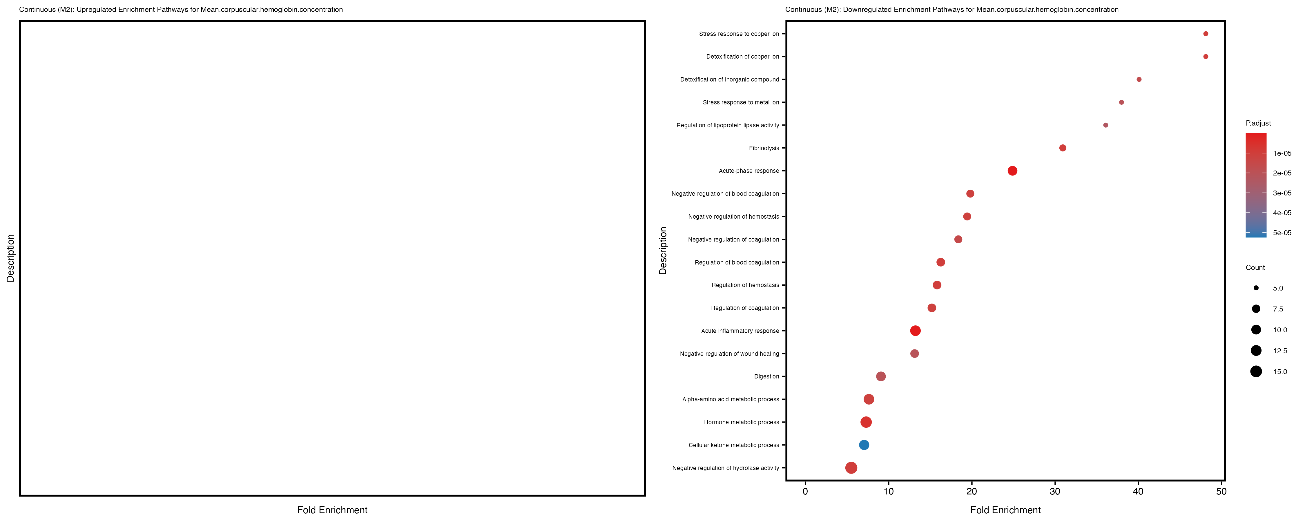
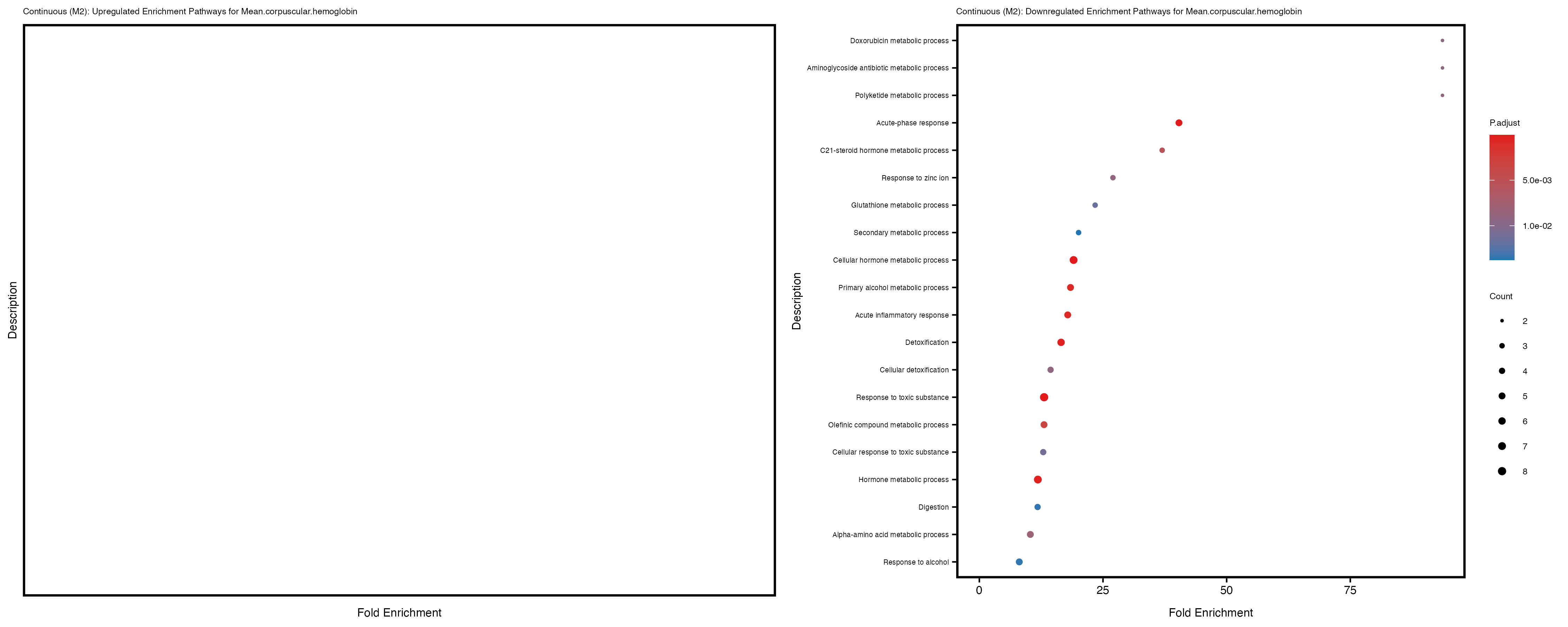
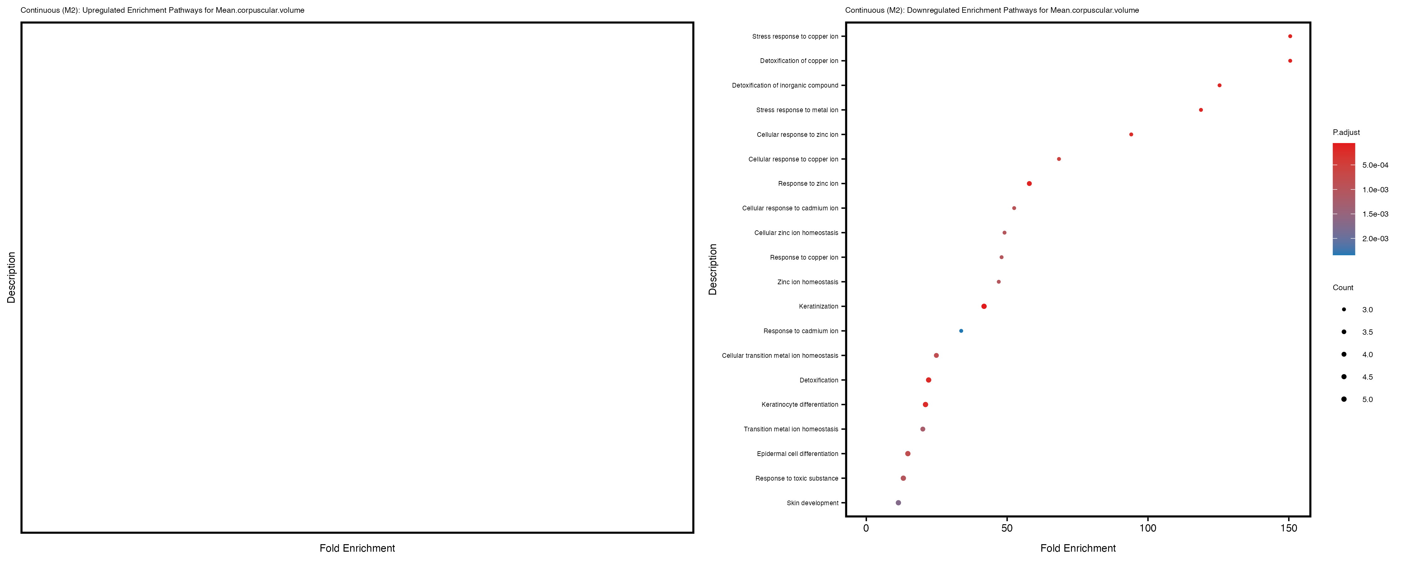
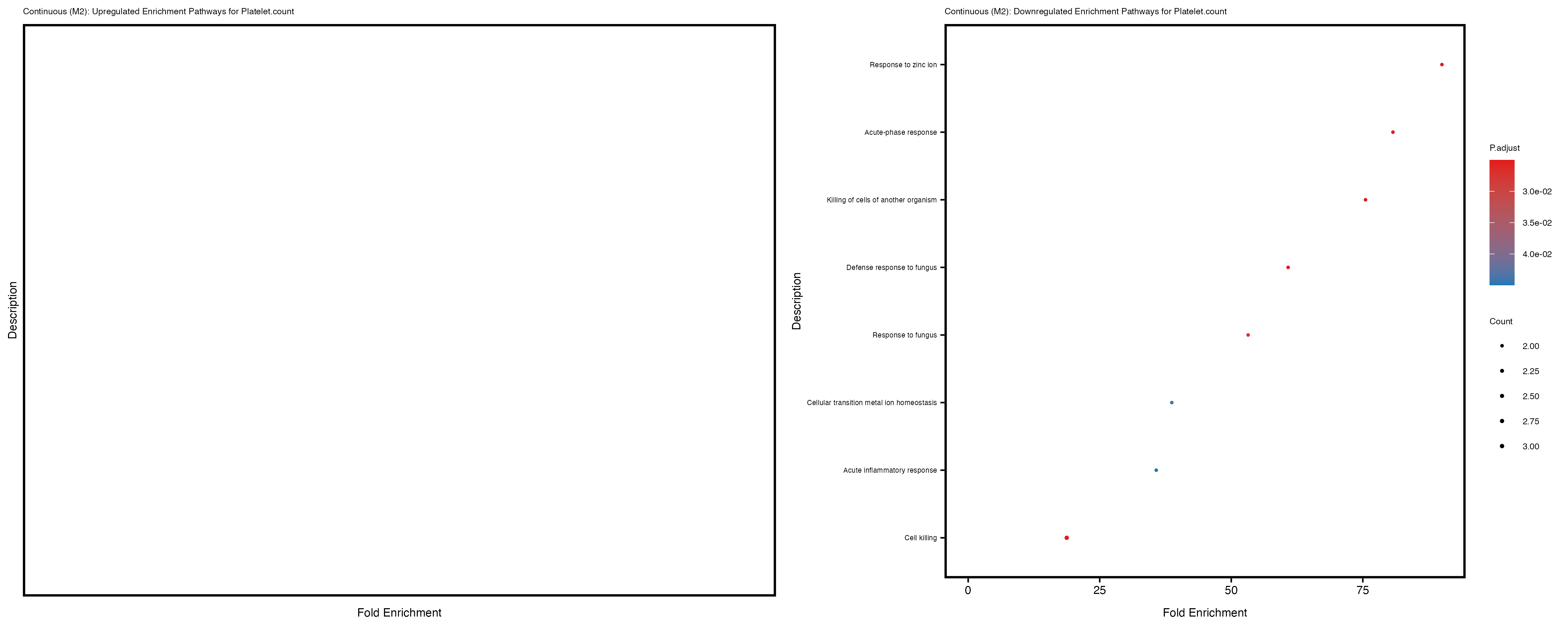
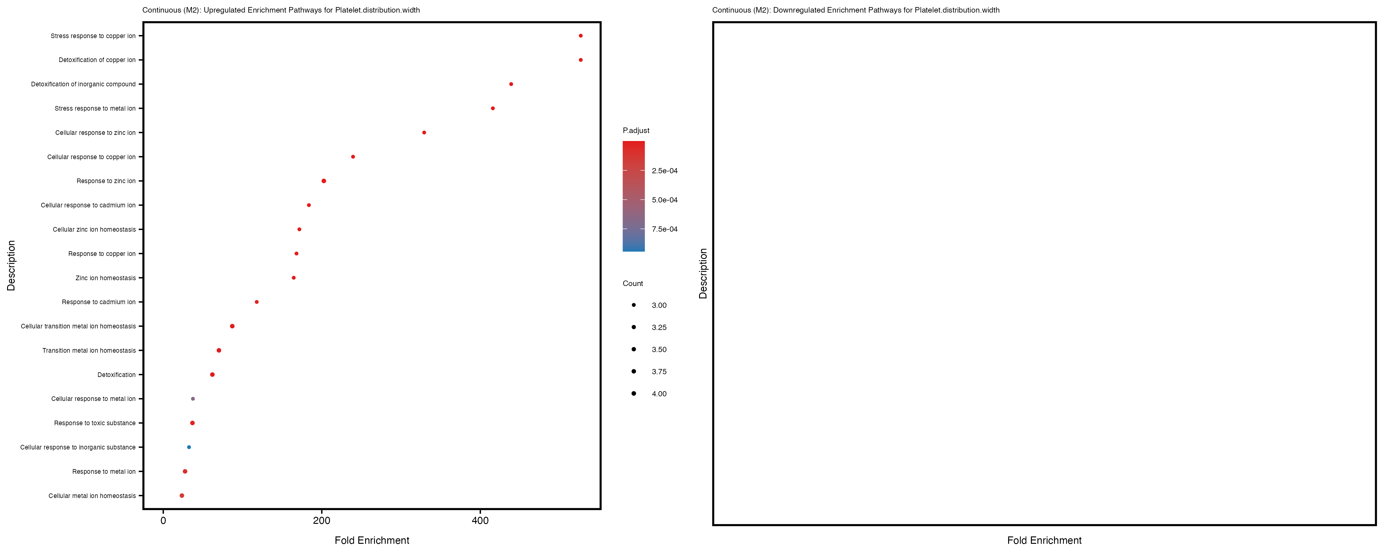
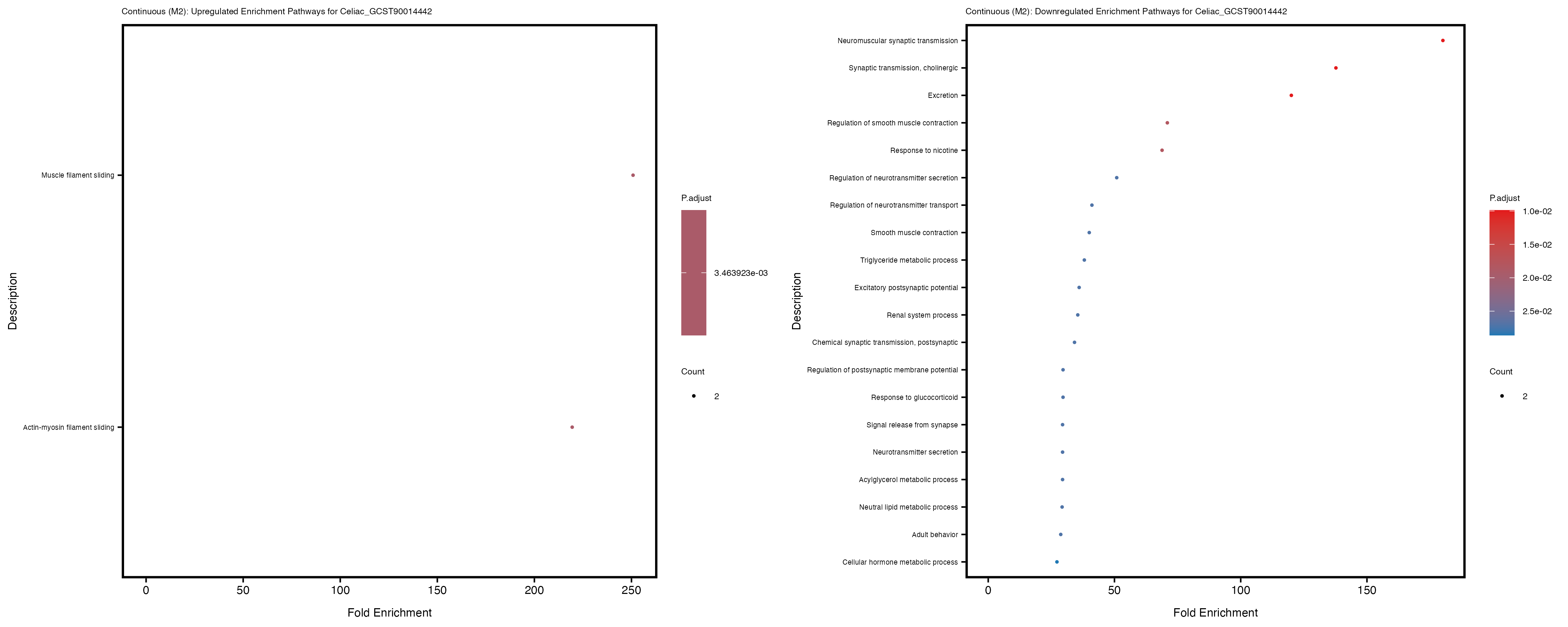
    labs(title = paste("Continuous: Downregulated Enrichment Pathways for", trait)) +
    theme(plot.title = element_text(size = 6), axis.text.y   = element_text(size = 5))
} else {
  enrich_plot_down <- plotEnrich(gse_down, plot_type = "dot", scale_ratio = 0.4) +
    labs(title = paste("Continuous: Downregulated Enrichment Pathways for", trait)) +
    theme(plot.title = element_text(size = 6), axis.text.y   = element_text(size = 5))
}
  
  # Arrange the two plots side by side
  combined_plot <- grid.arrange(enrich_plot_up, enrich_plot_down, ncol = 2)
  
  # Save the combined plot
  ggsave(paste0("enrichment_plot_", trait, ".png"), plot = combined_plot, 
         width = 15, height = 6)
  
  # Save the GO enrichment results to CSV
  write.csv(gse_up, file = paste0("GO_enrichment_", trait, "_upregulated.csv"))
  write.csv(gse_down, file = paste0("GO_enrichment_", trait, "_downregulated.csv"))
}

Quantile PRS:

dir_path <- "analysis/quantile_wb"
files <- list.files(dir_path, pattern = "differential_expression_.*_quantile_results.csv", 
                    full.names = TRUE)

for (file in files) {
  trait <- gsub("differential_expression_(.*)_quantile_results.csv", "\\1", basename(file))
  trait
  res_tableOE <- read.csv(file, header = T, row.names = 1)
  
  deGenes <- res_tableOE[res_tableOE$padj < 0.1 & 
                           abs(res_tableOE$log2FoldChange) >= 0.5, ]
  deGenes$gene_id <- gsub("\\.\\d+$", "", rownames(deGenes))
  
  # Separate upregulated and downregulated genes
  upregulated_genes <- deGenes[deGenes$log2FoldChange > 0, ]$gene_id
  downregulated_genes <- deGenes[deGenes$log2FoldChange < 0, ]$gene_id
  
  # Run GO enrichment for upregulated genes
  gse_up <- enrichGO(gene = upregulated_genes, ont = "BP", 
                   OrgDb = "org.Hs.eg.db", keyType = "ENSEMBL", readable = T)
  
  # Run GO enrichment for downregulated genes
  gse_down <- enrichGO(gene = downregulated_genes, ont = "BP", 
                     OrgDb = "org.Hs.eg.db", keyType = "ENSEMBL", readable = T)
  
  # Convert enrichment results to data frames and calculate additional ratios
  if (is.null(gse_up)) {
    gse_up <- data.frame(ID = character(), Description = character(),
                       GeneRatio = character(), BgRatio = character(),
                       pvalue = numeric(), p.adjust = numeric(),
                       qvalue = numeric(), geneID = character(),
                       Count = integer(), stringsAsFactors = FALSE)
  } else { 
    gse_up <- as.data.frame(gse_up)}
  
  gse_down <- as.data.frame(gse_down)
  
  gse_up$GeneRatio_num <- as.numeric(sapply(strsplit(gse_up$GeneRatio, "/"), function(x) x[1])) / 
                        as.numeric(sapply(strsplit(gse_up$GeneRatio, "/"), function(x) x[2]))
  gse_up$BgRatio_num <- as.numeric(sapply(strsplit(gse_up$BgRatio, "/"), function(x) x[1])) / 
                        as.numeric(sapply(strsplit(gse_up$BgRatio, "/"), function(x) x[2]))
  gse_up <- cbind(gse_up, FoldEnrich = gse_up$GeneRatio_num / gse_up$BgRatio_num)

  gse_down$GeneRatio_num <- as.numeric(sapply(strsplit(gse_down$GeneRatio, "/"), function(x) x[1])) / 
                          as.numeric(sapply(strsplit(gse_down$GeneRatio, "/"), function(x) x[2]))
  gse_down$BgRatio_num <- as.numeric(sapply(strsplit(gse_down$BgRatio, "/"), function(x) x[1])) / 
                          as.numeric(sapply(strsplit(gse_down$BgRatio, "/"), function(x) x[2]))
  gse_down <- cbind(gse_down, FoldEnrich = gse_down$GeneRatio_num / gse_down$BgRatio_num)
  
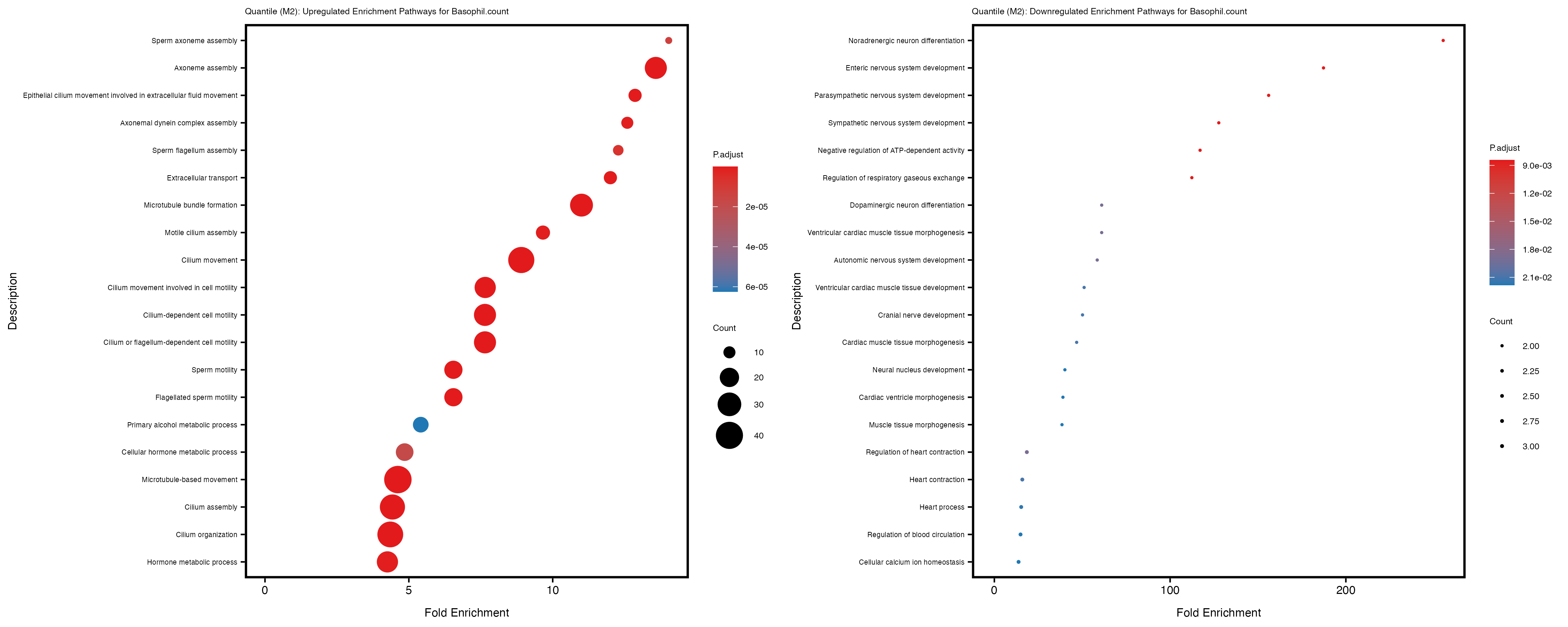
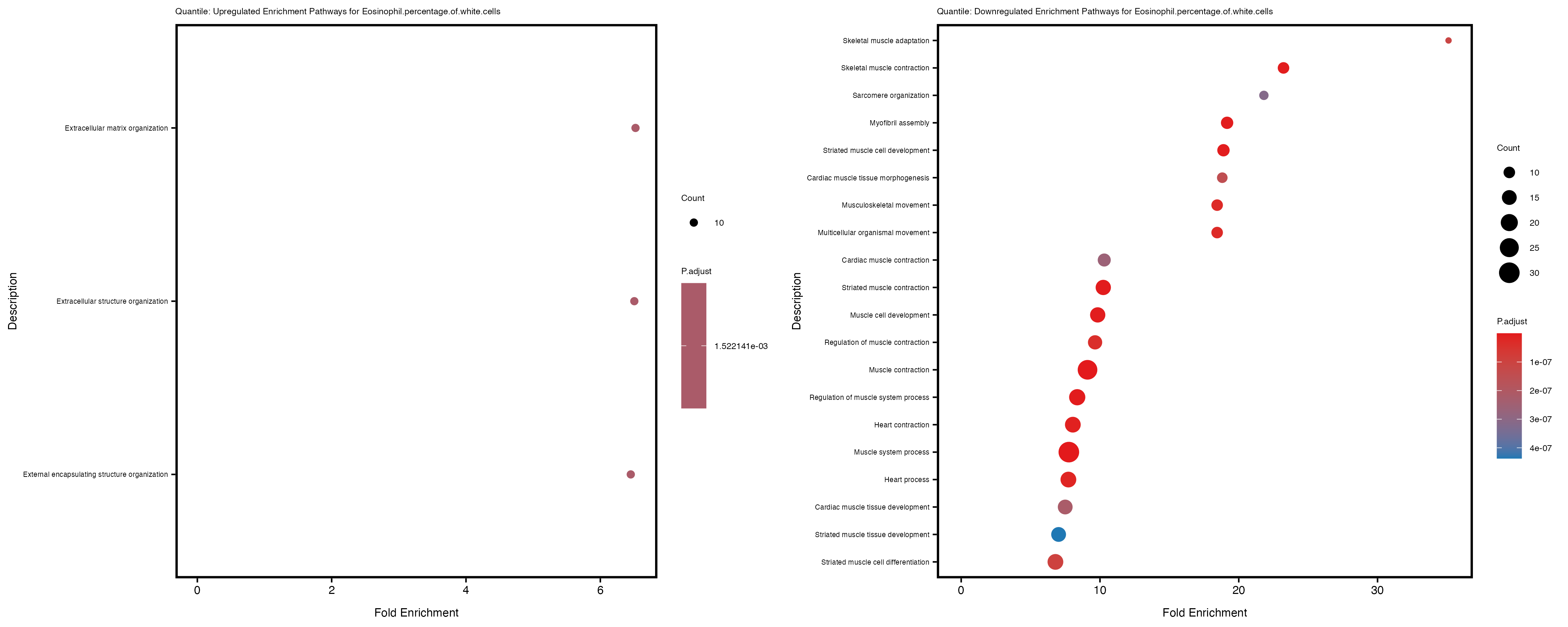
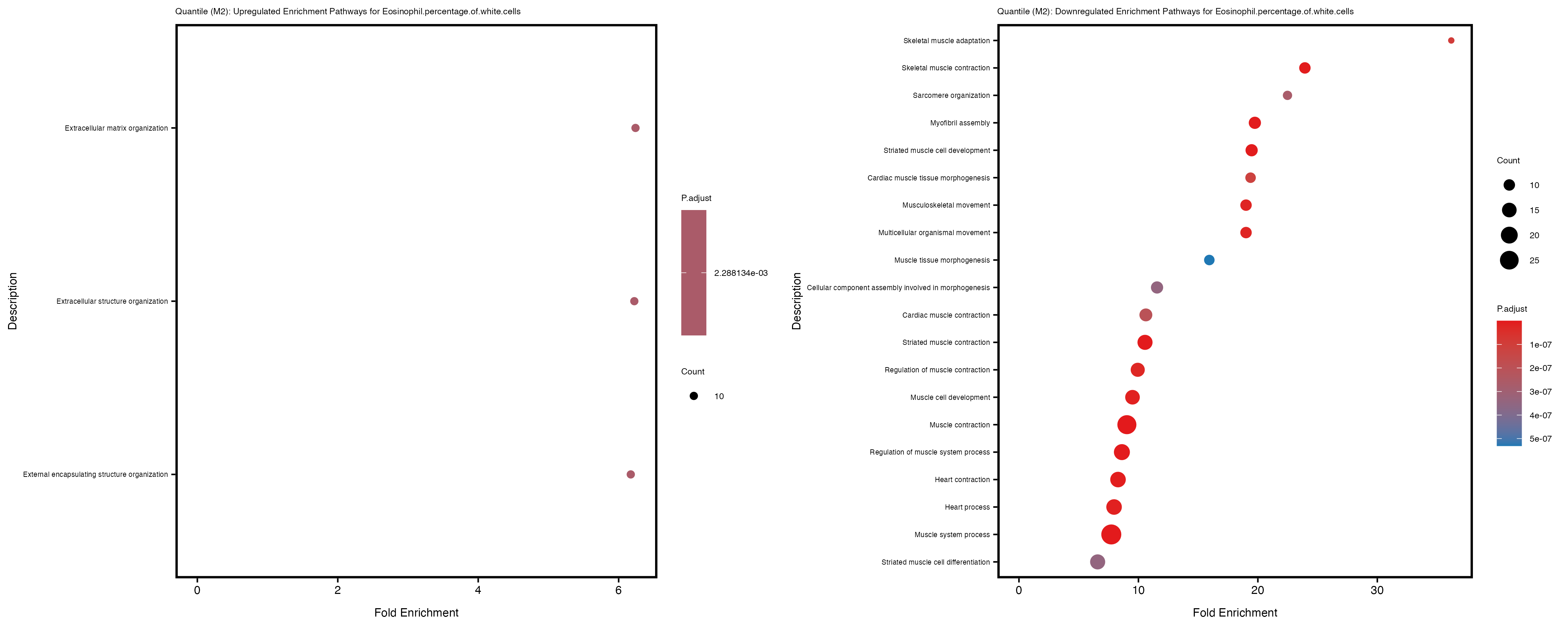
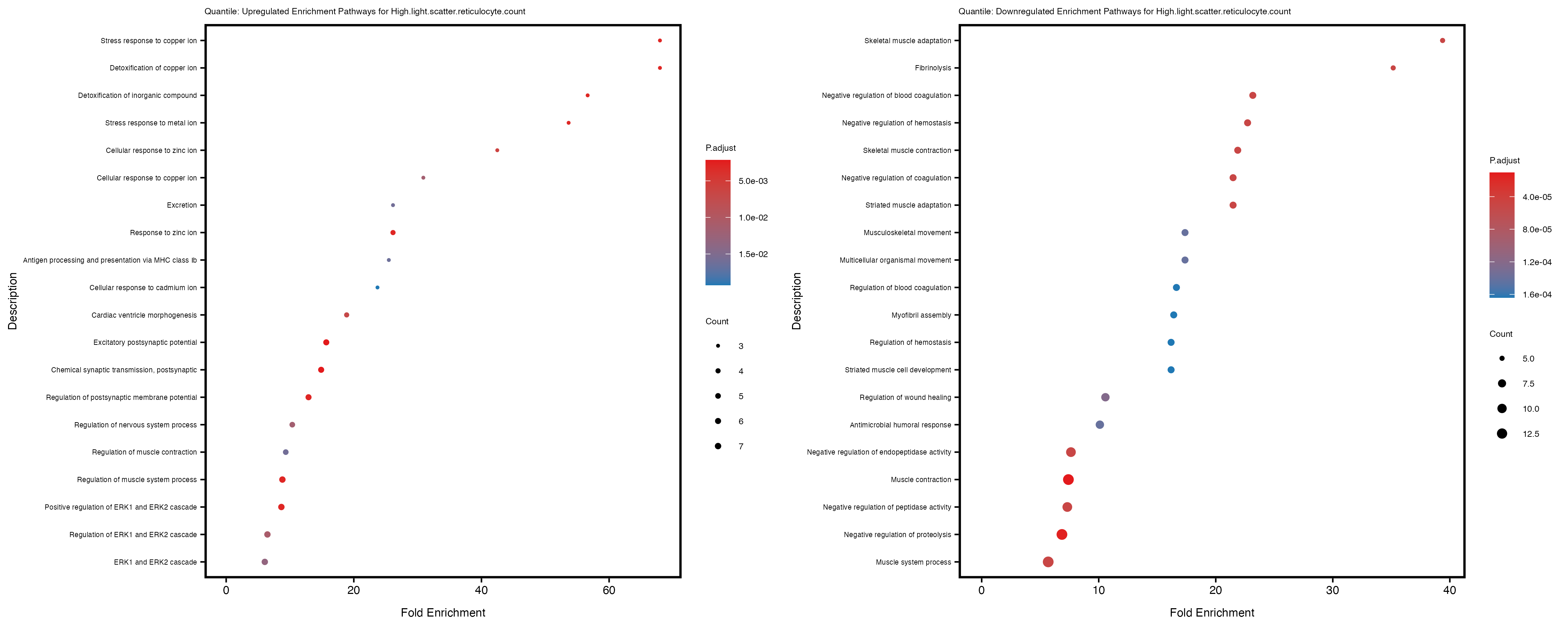
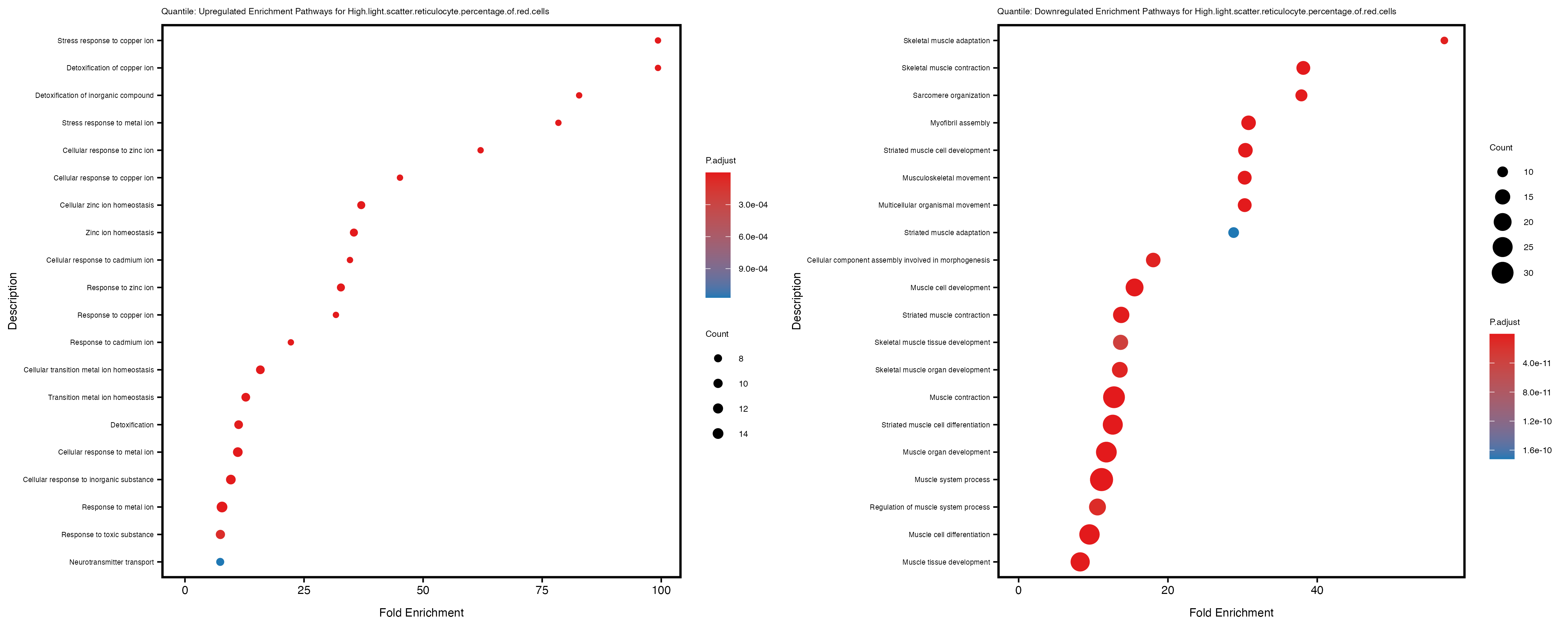
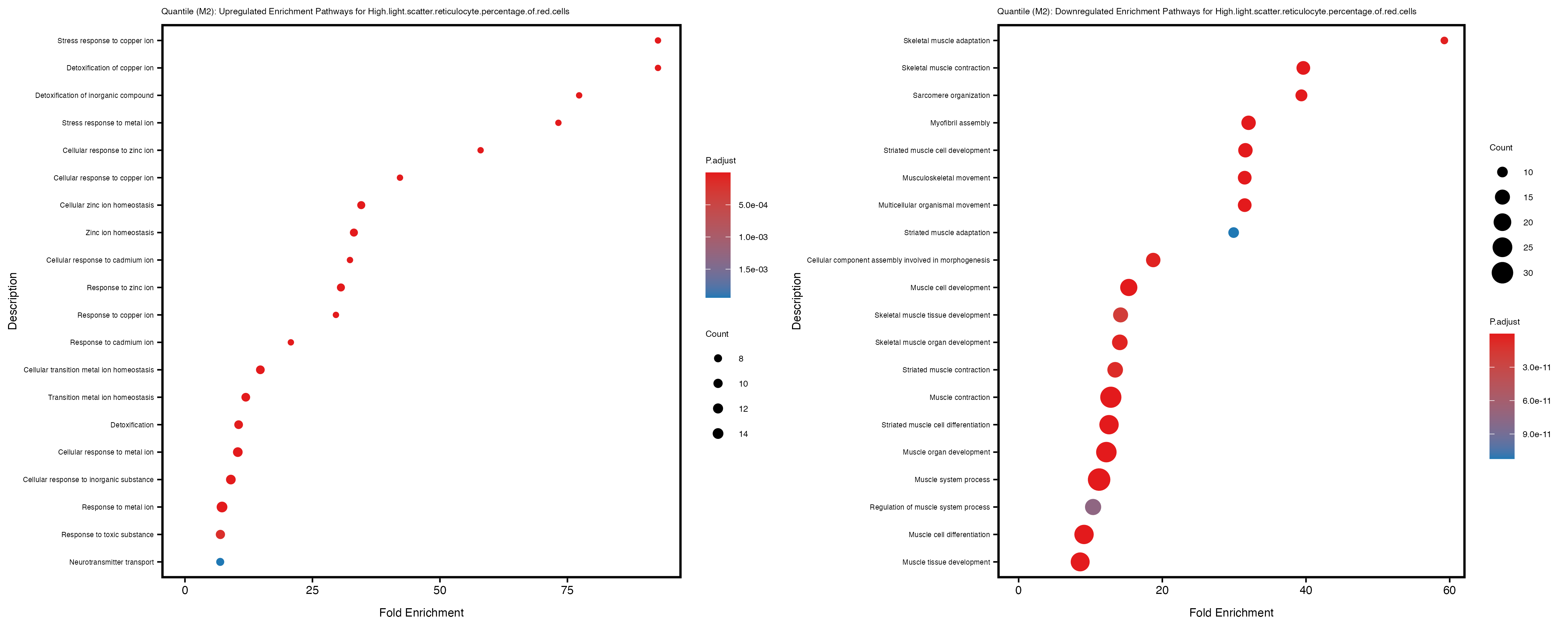
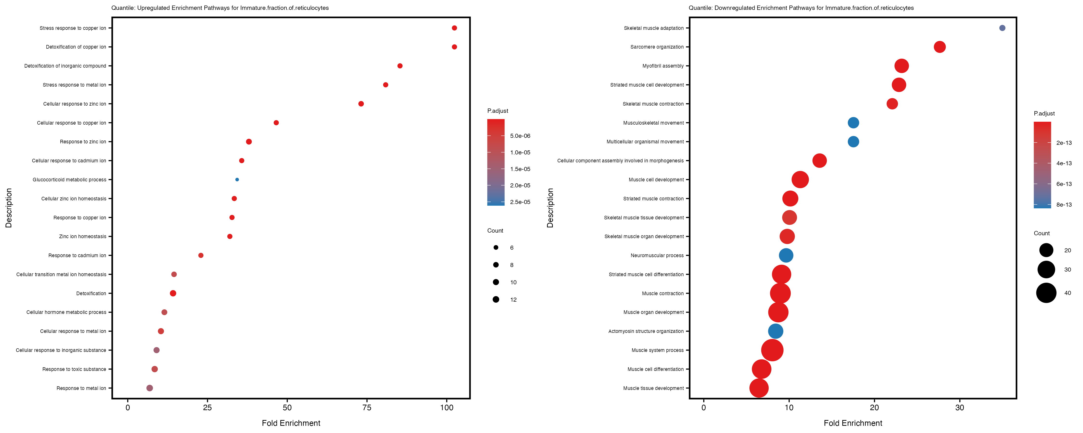
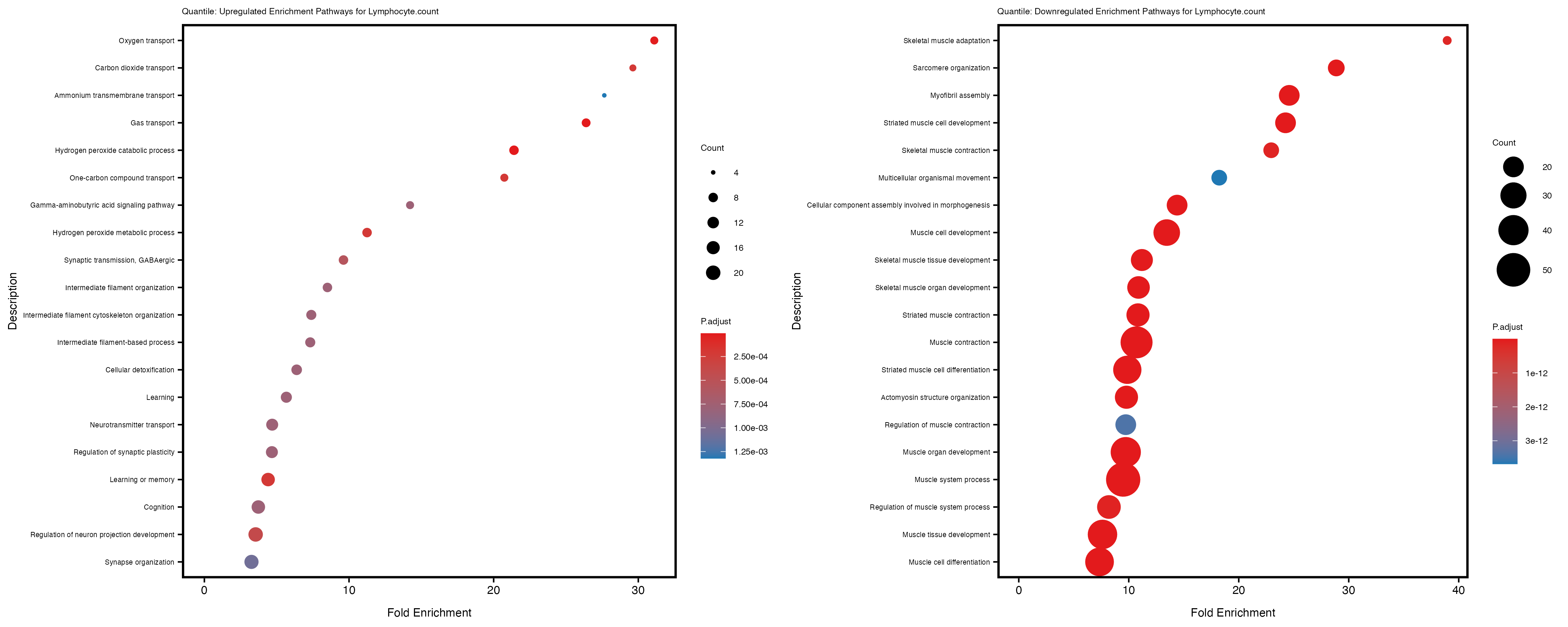
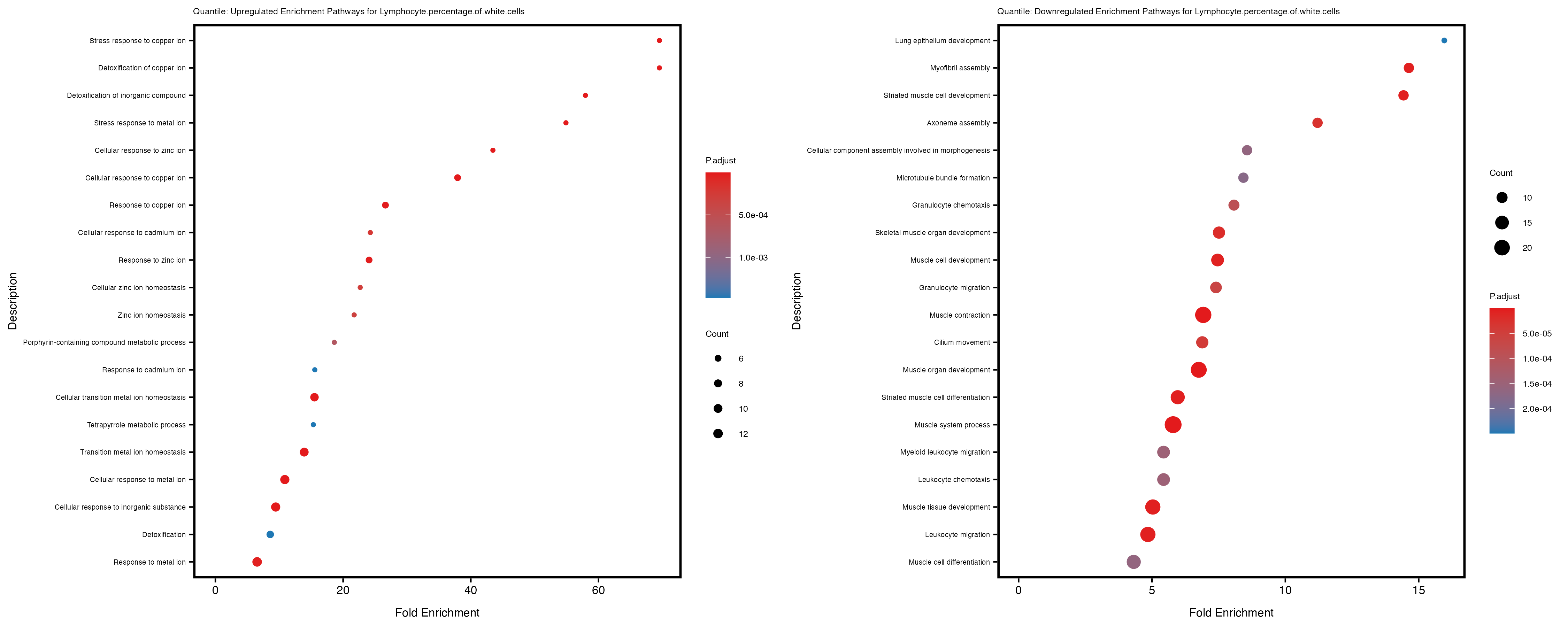
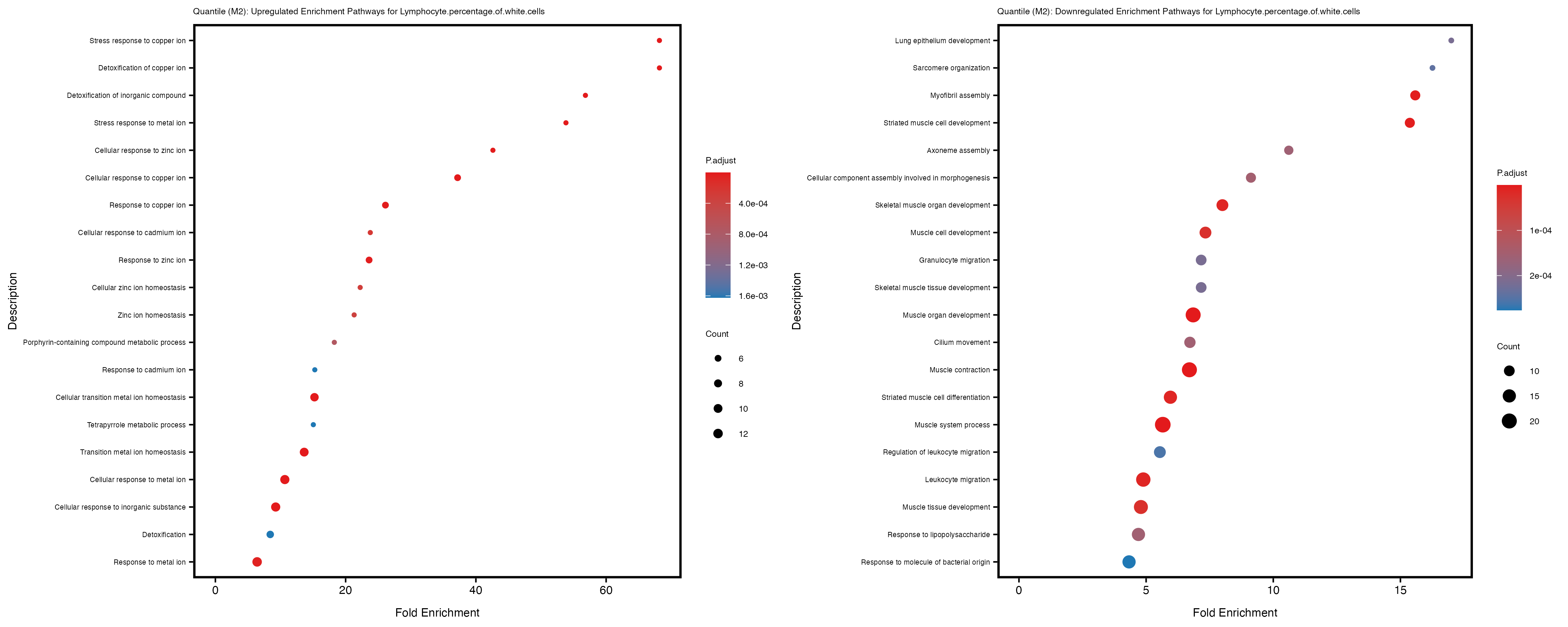
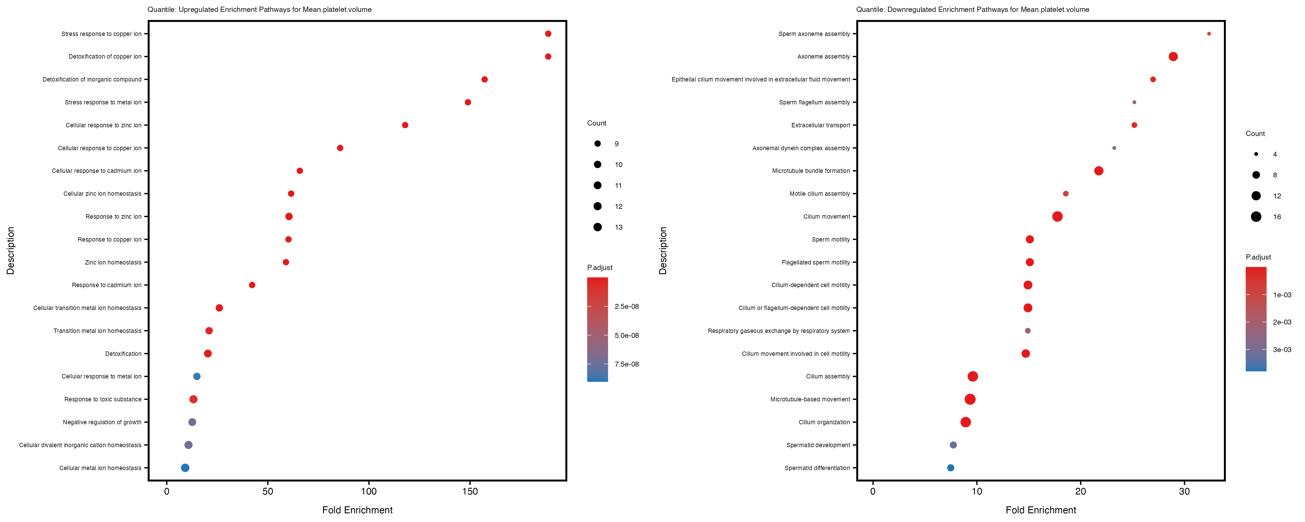
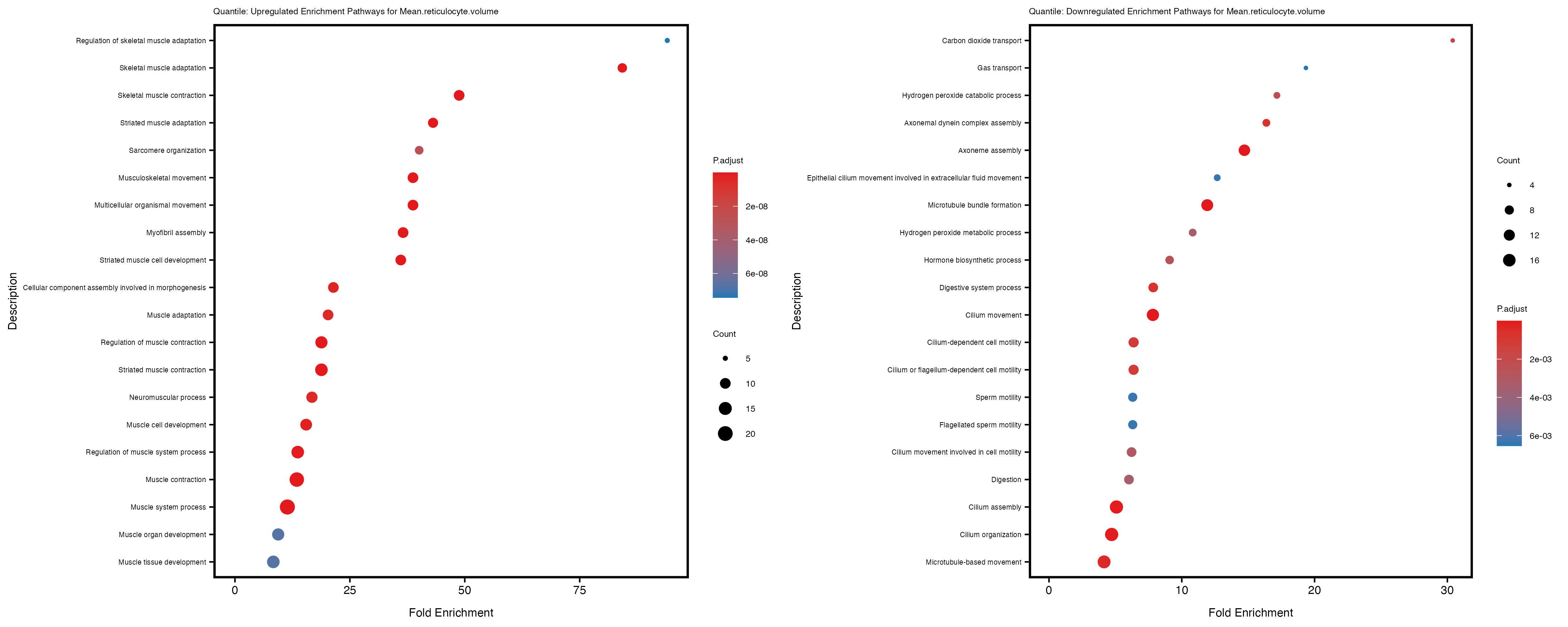
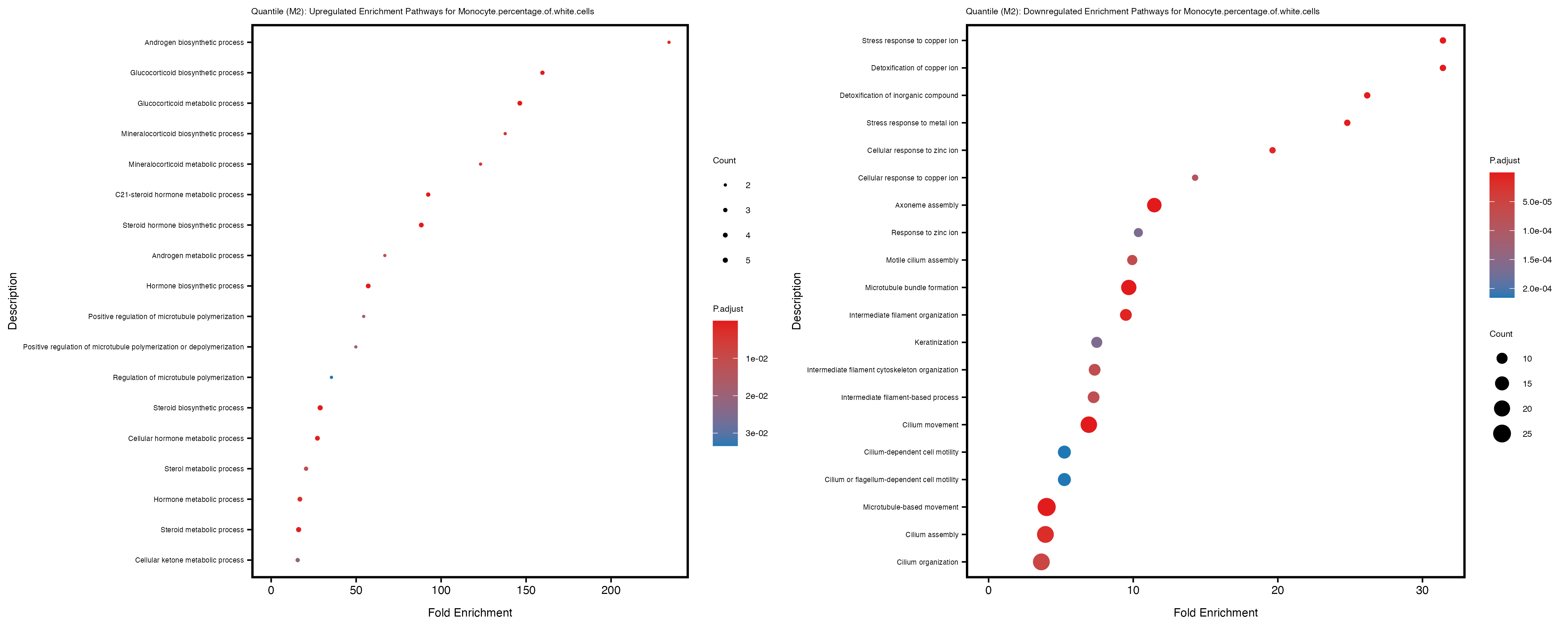
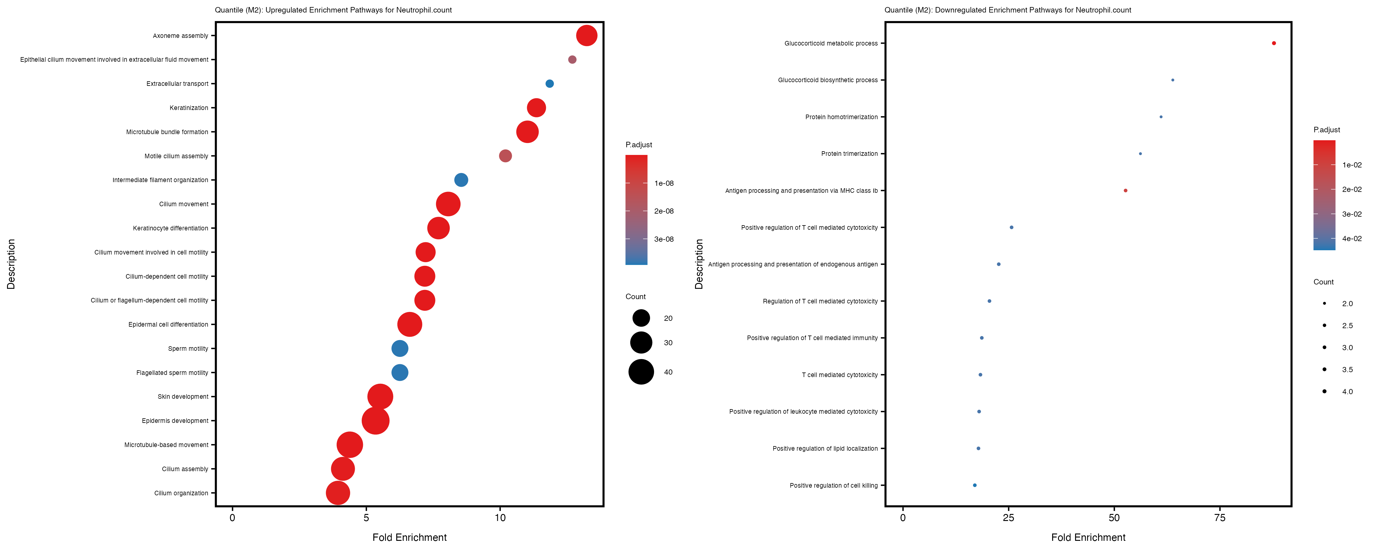
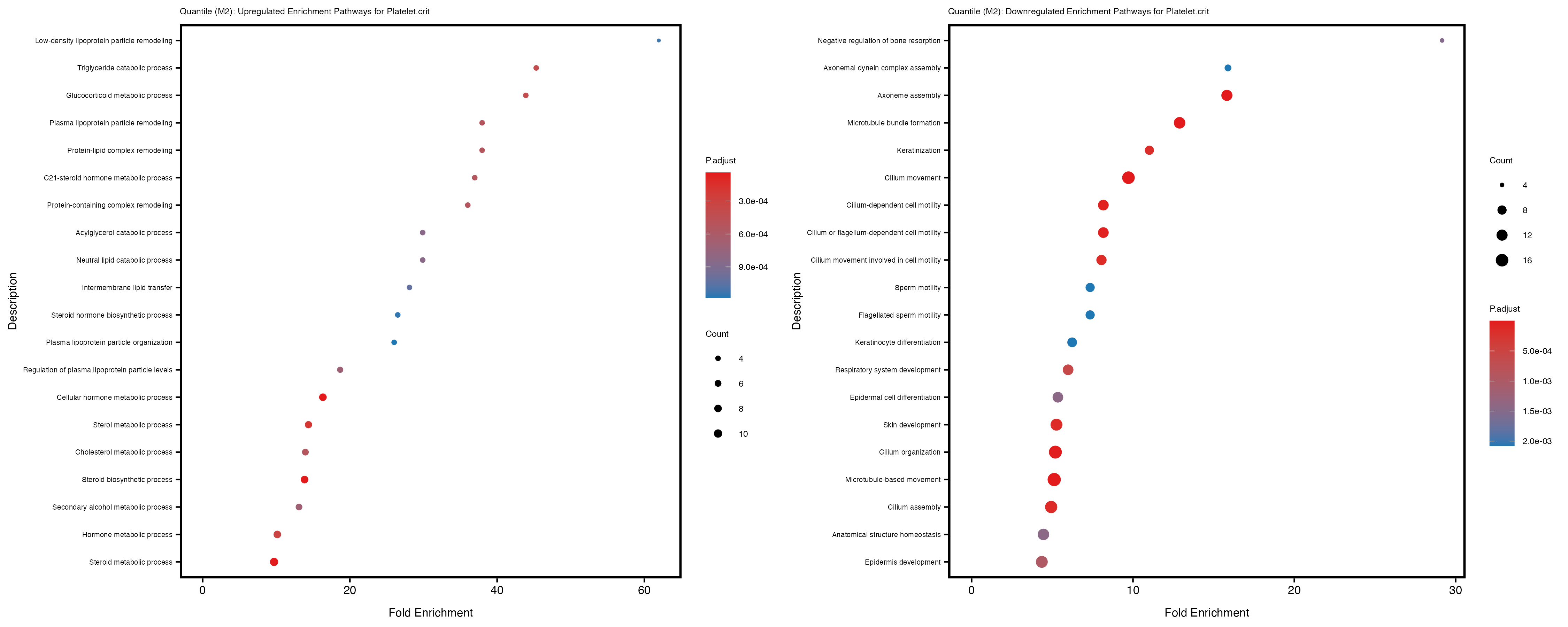
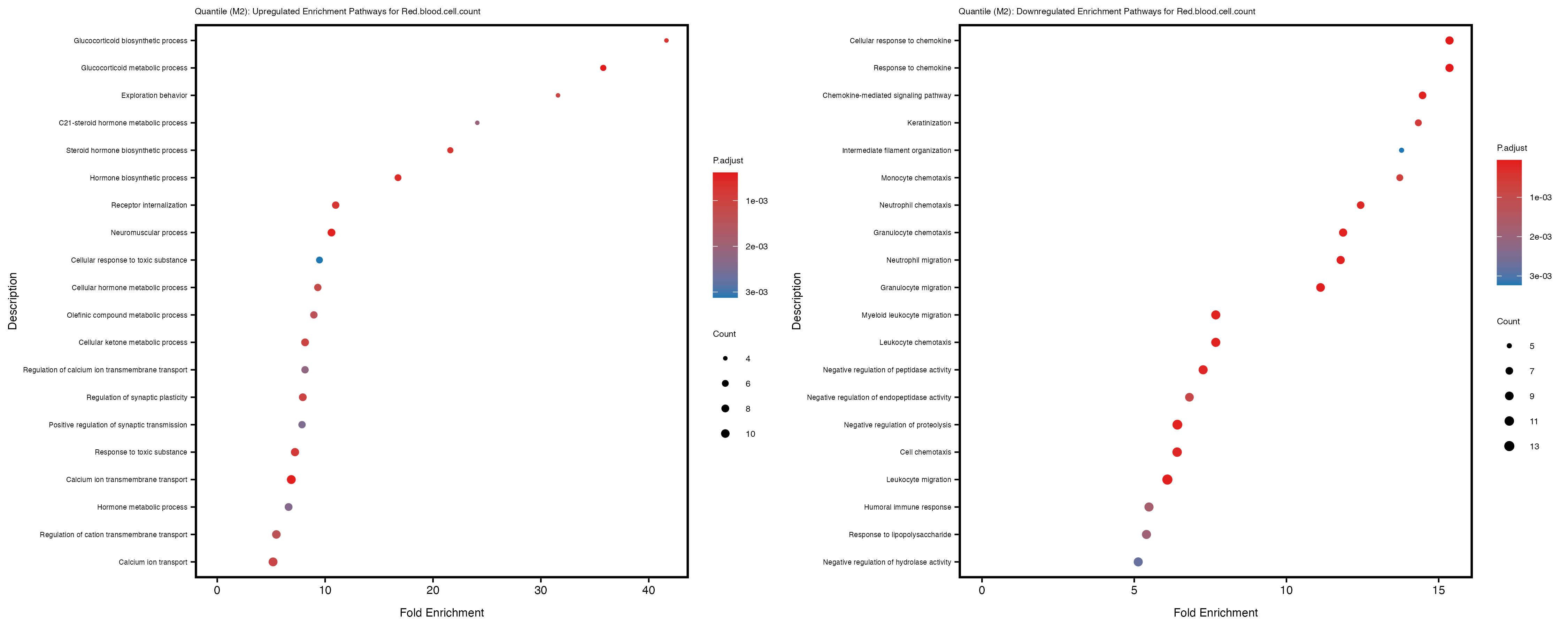
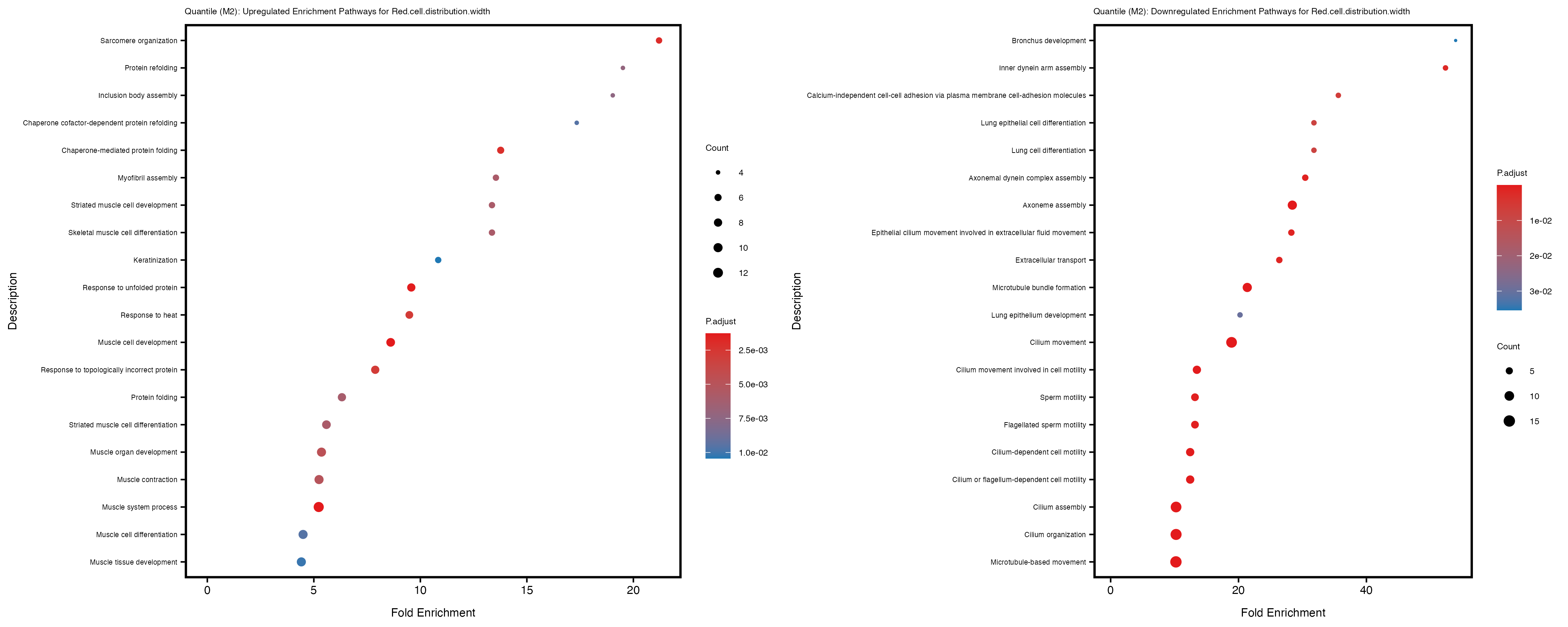
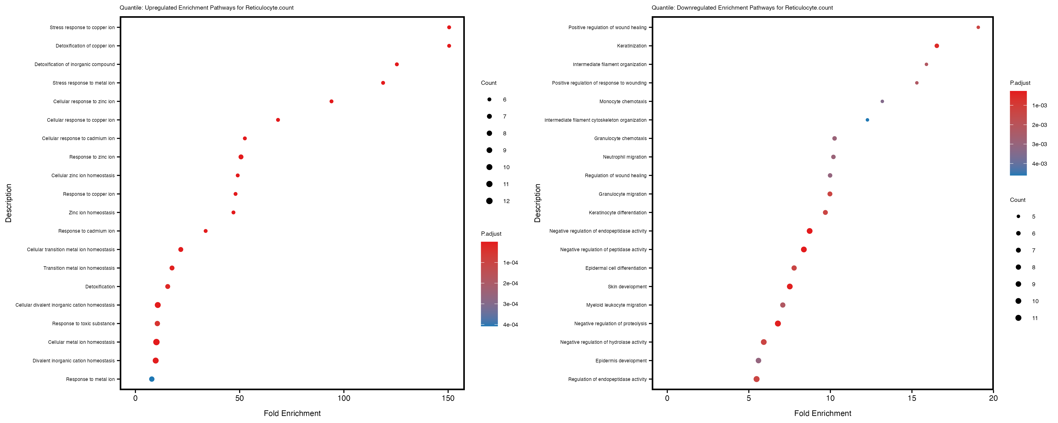
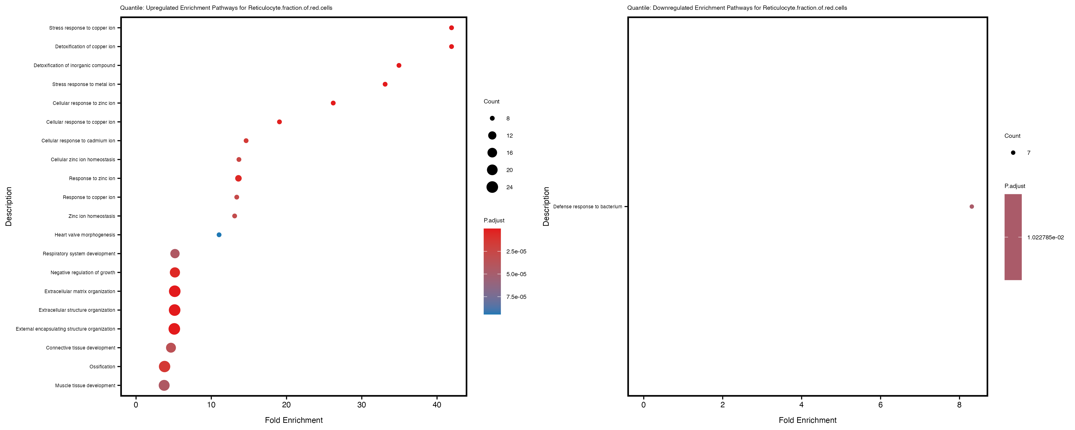
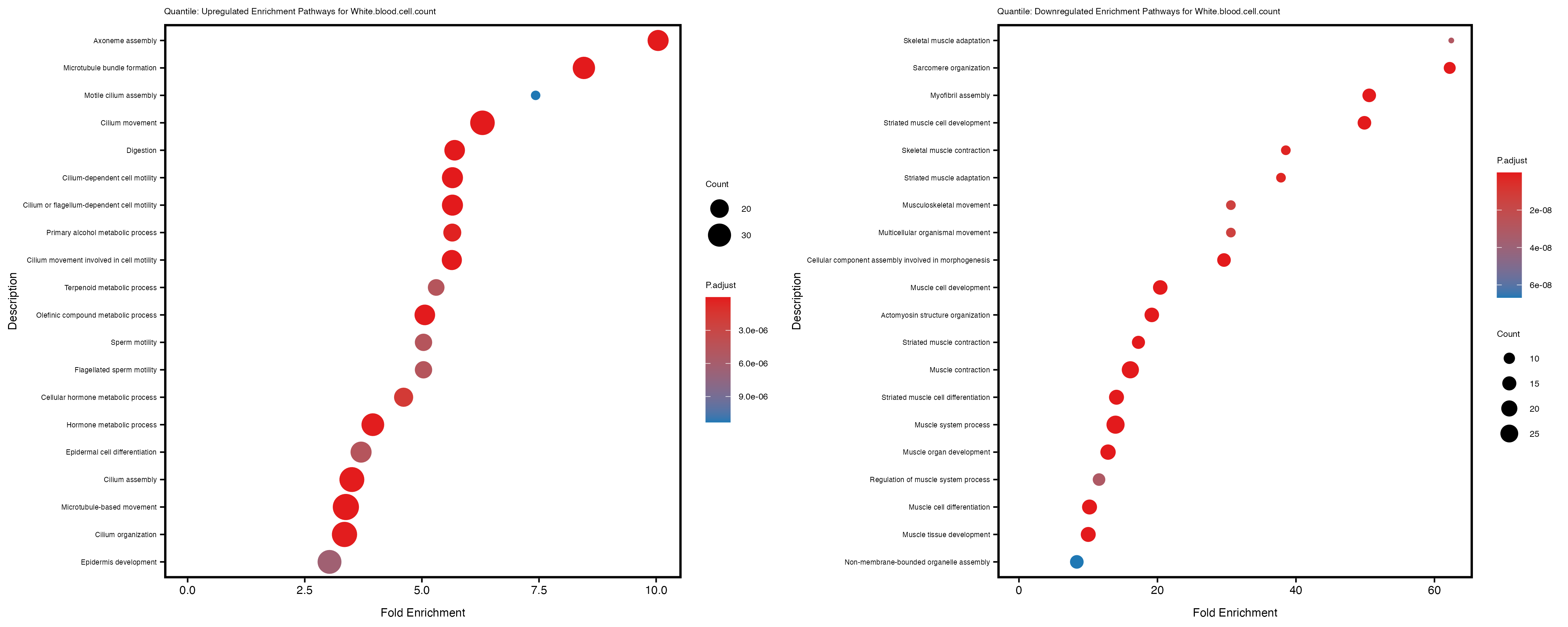
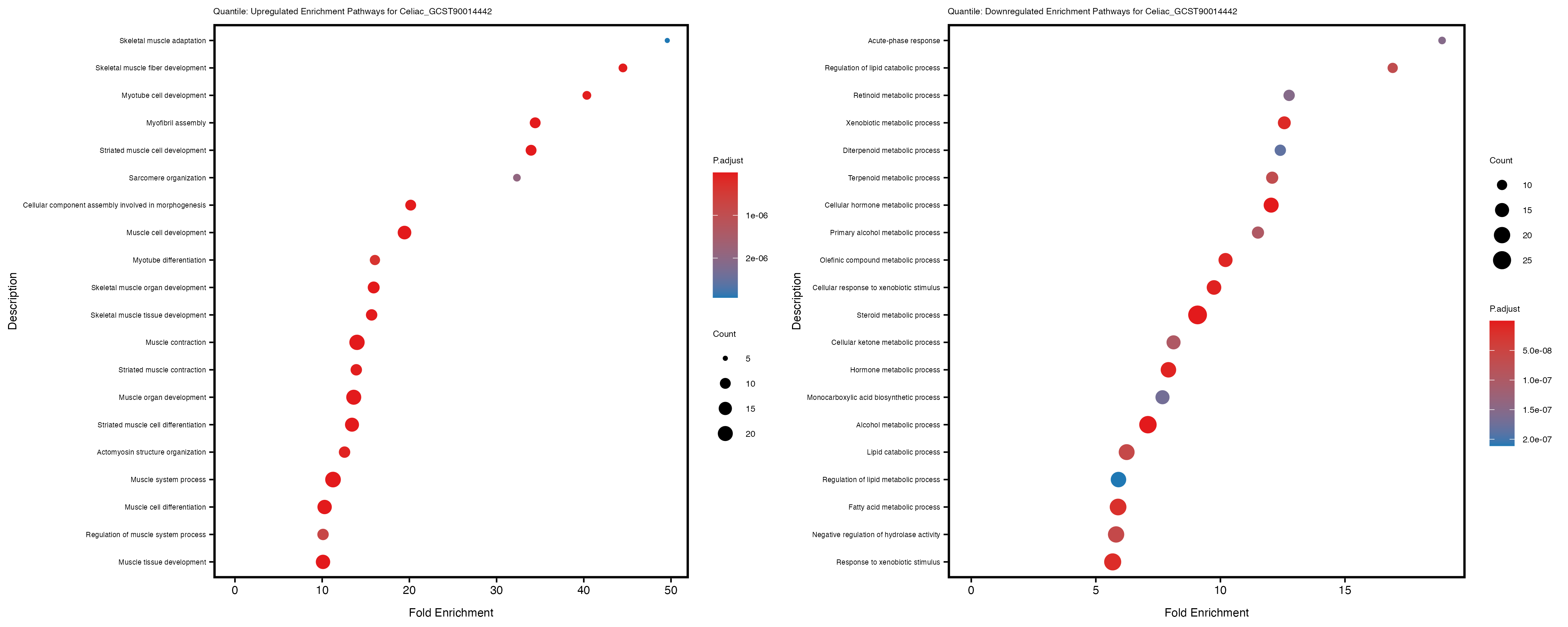
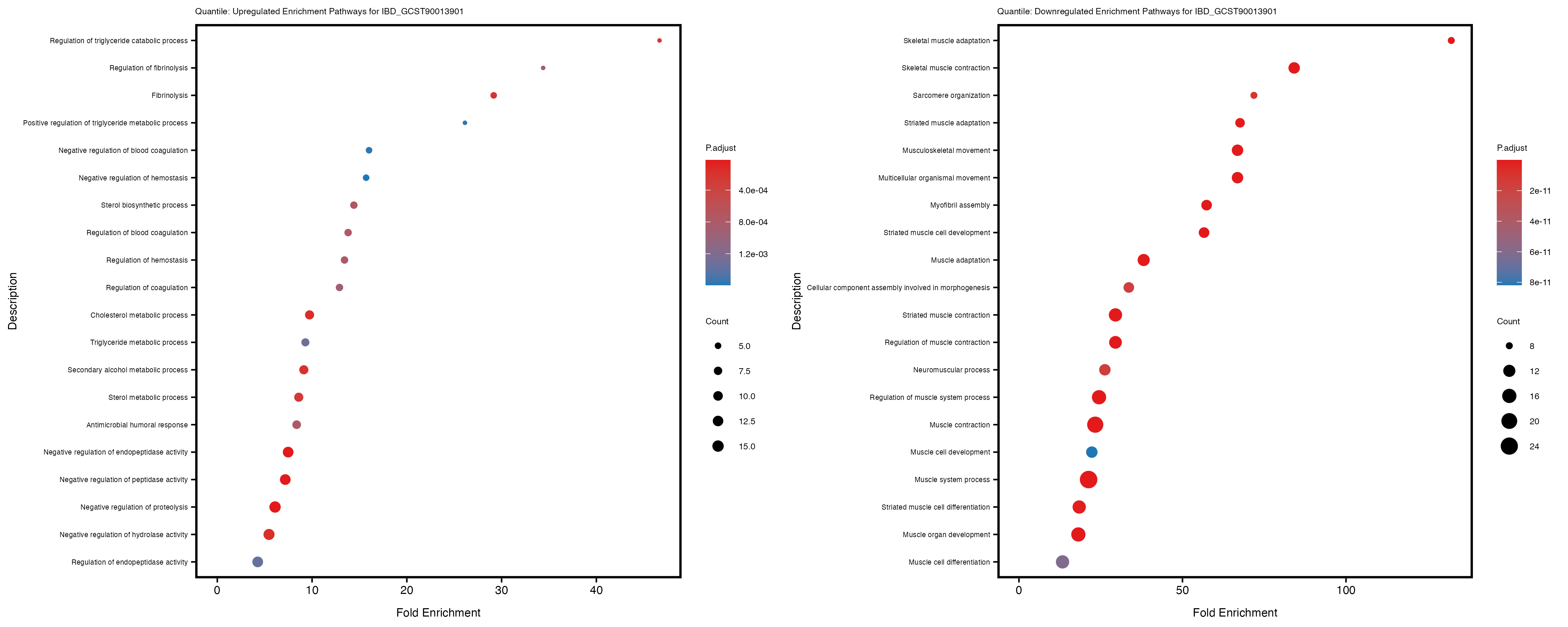
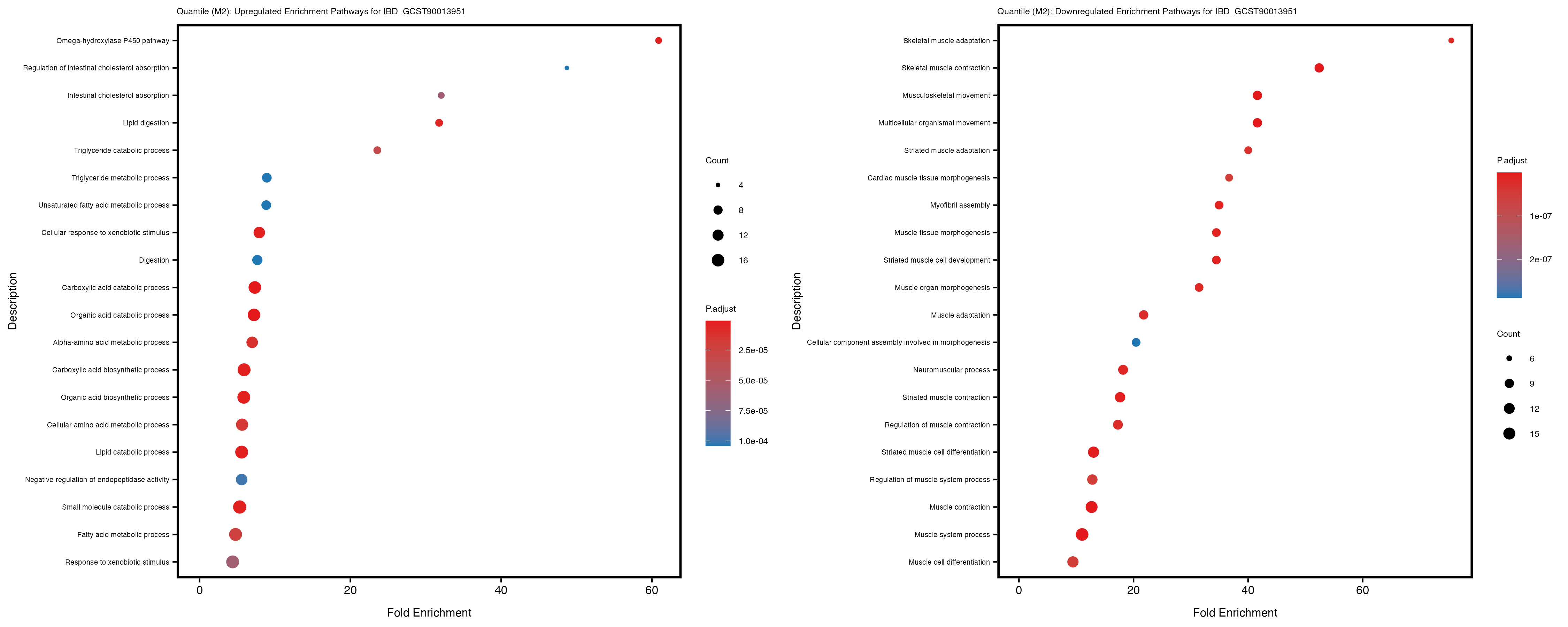
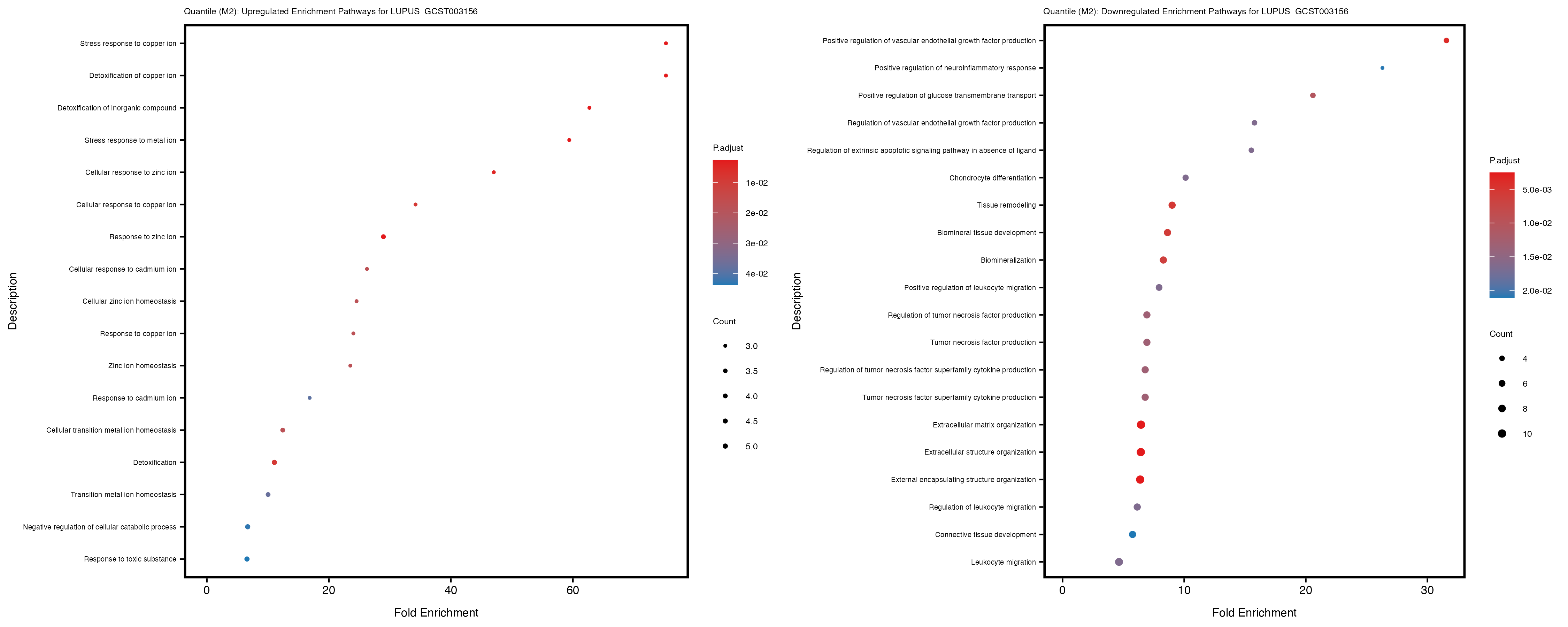
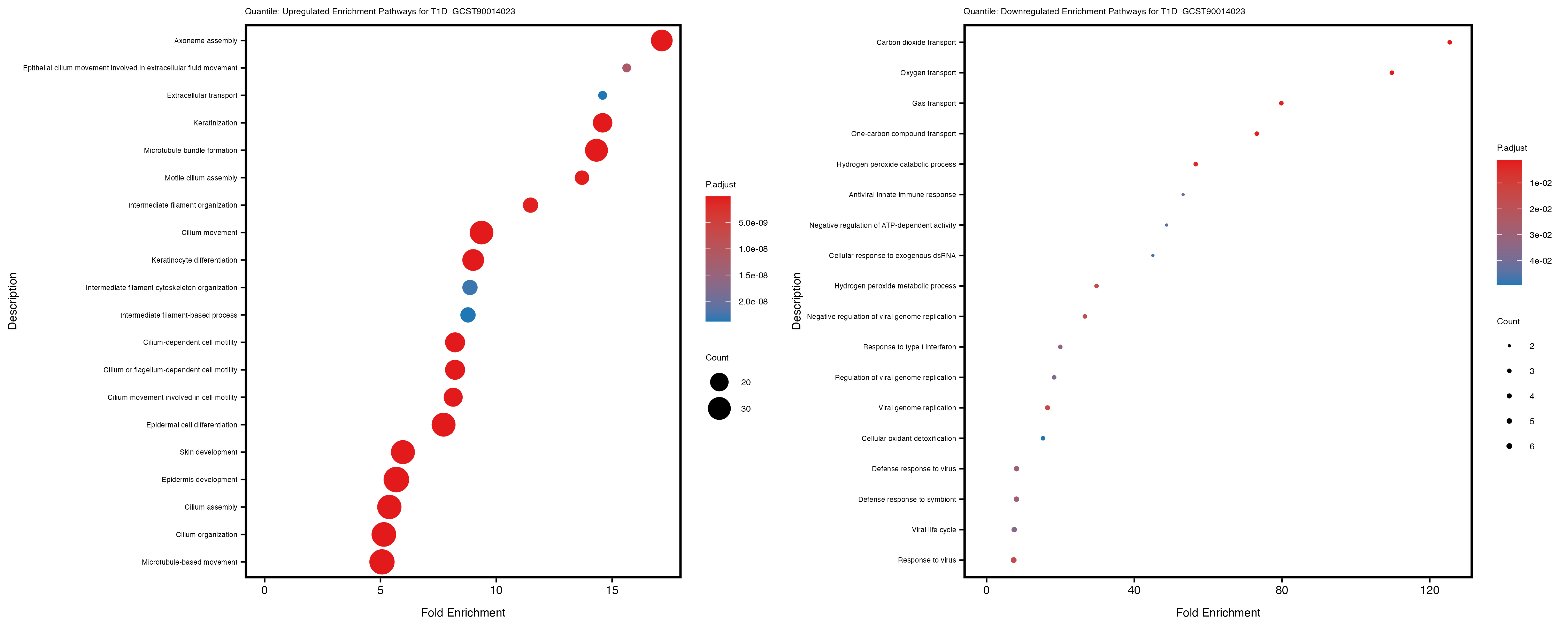
if (nrow(gse_up) >= 20) {
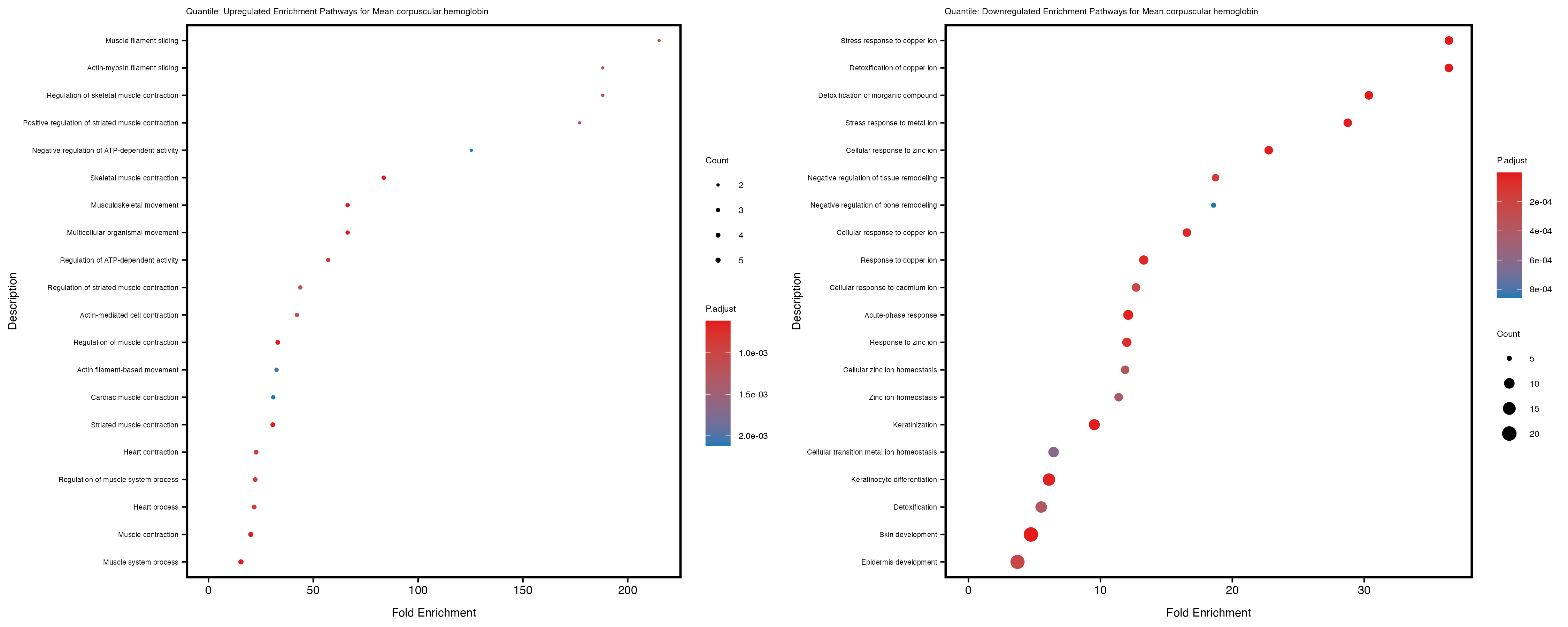
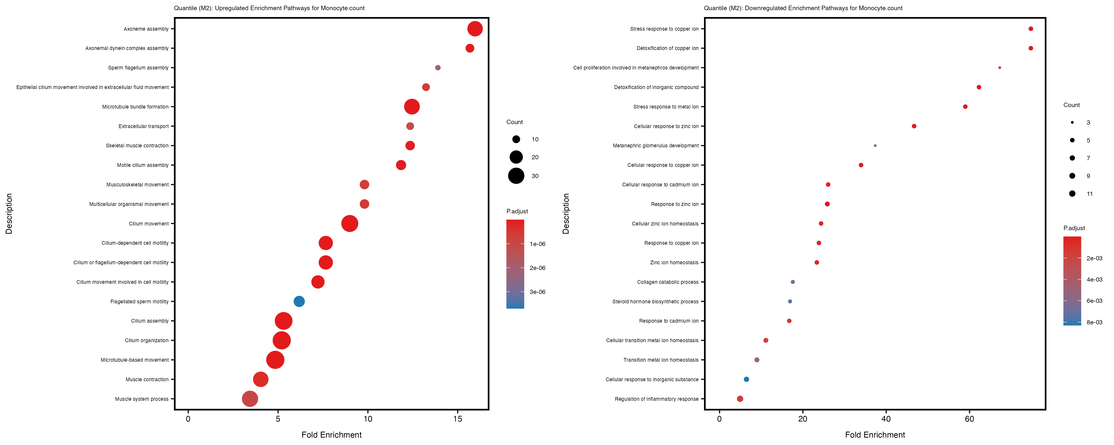
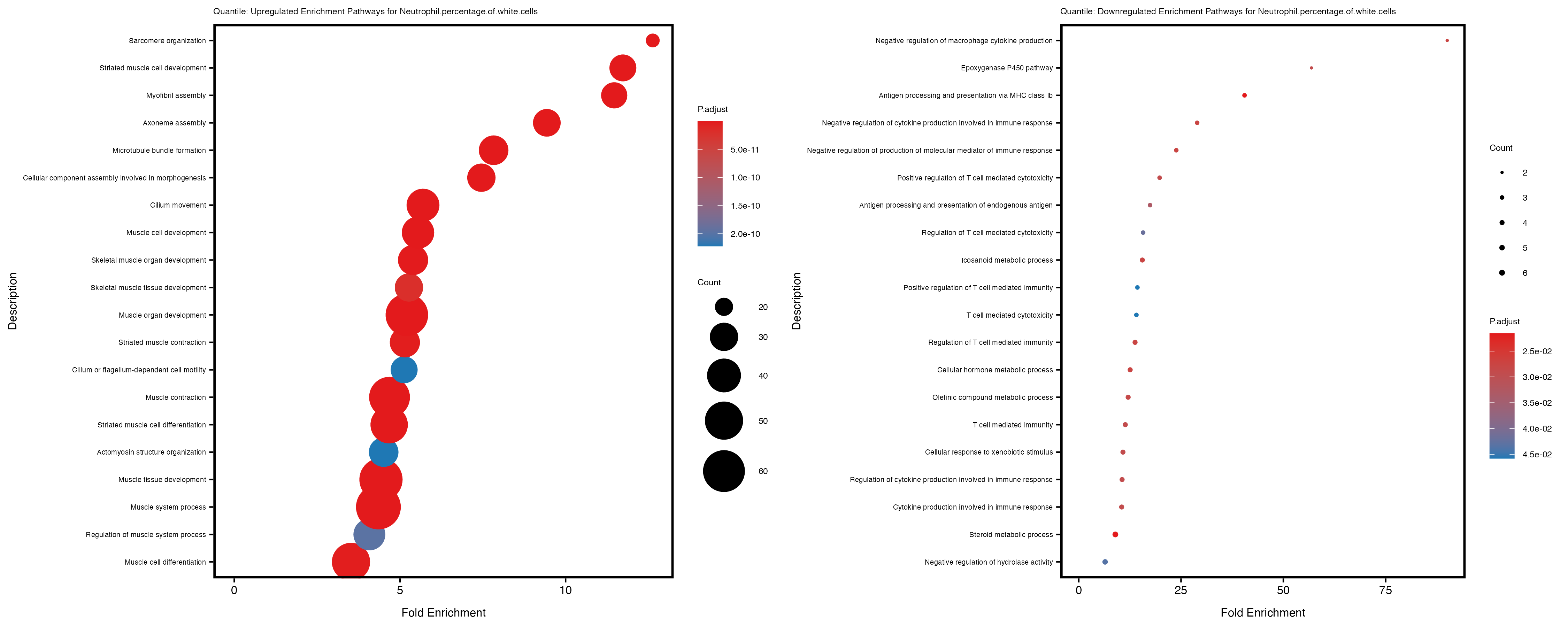
  enrich_plot_up <- plotEnrich(gse_up[1:20, ], plot_type = "dot", scale_ratio = 0.4) +
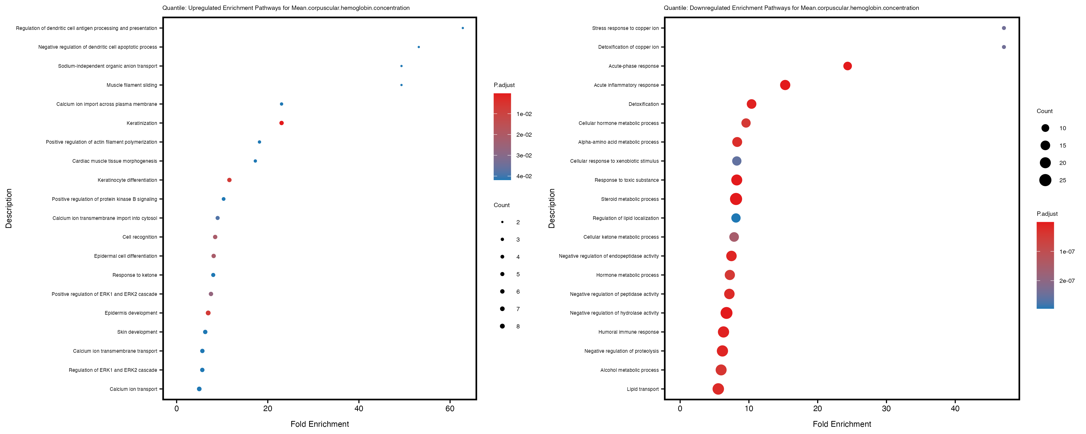
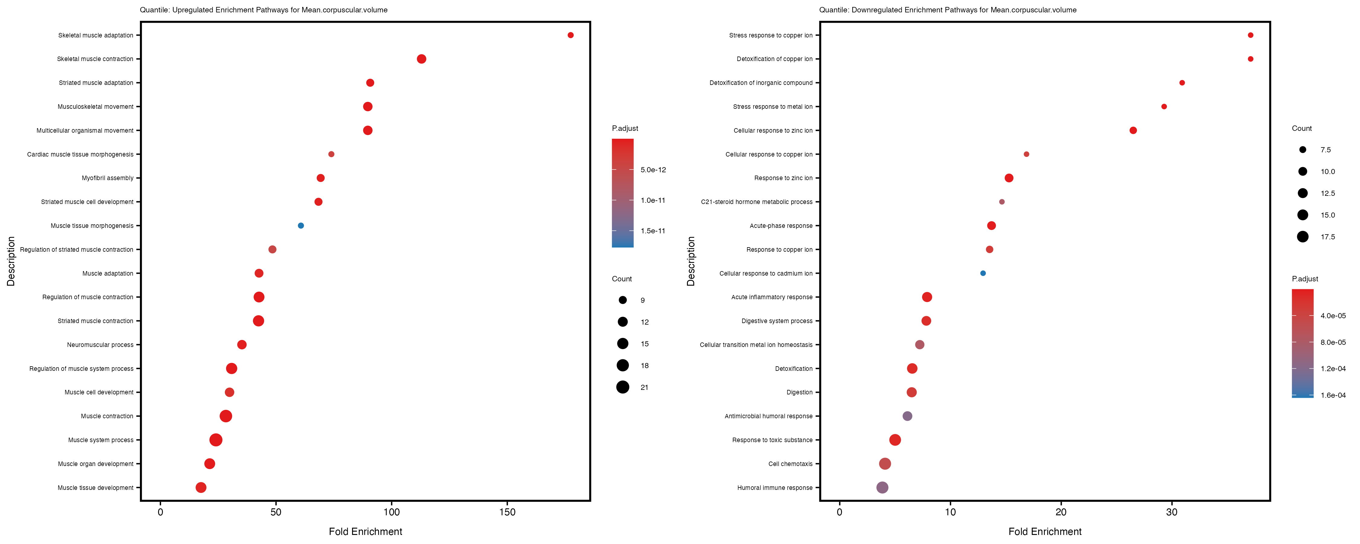
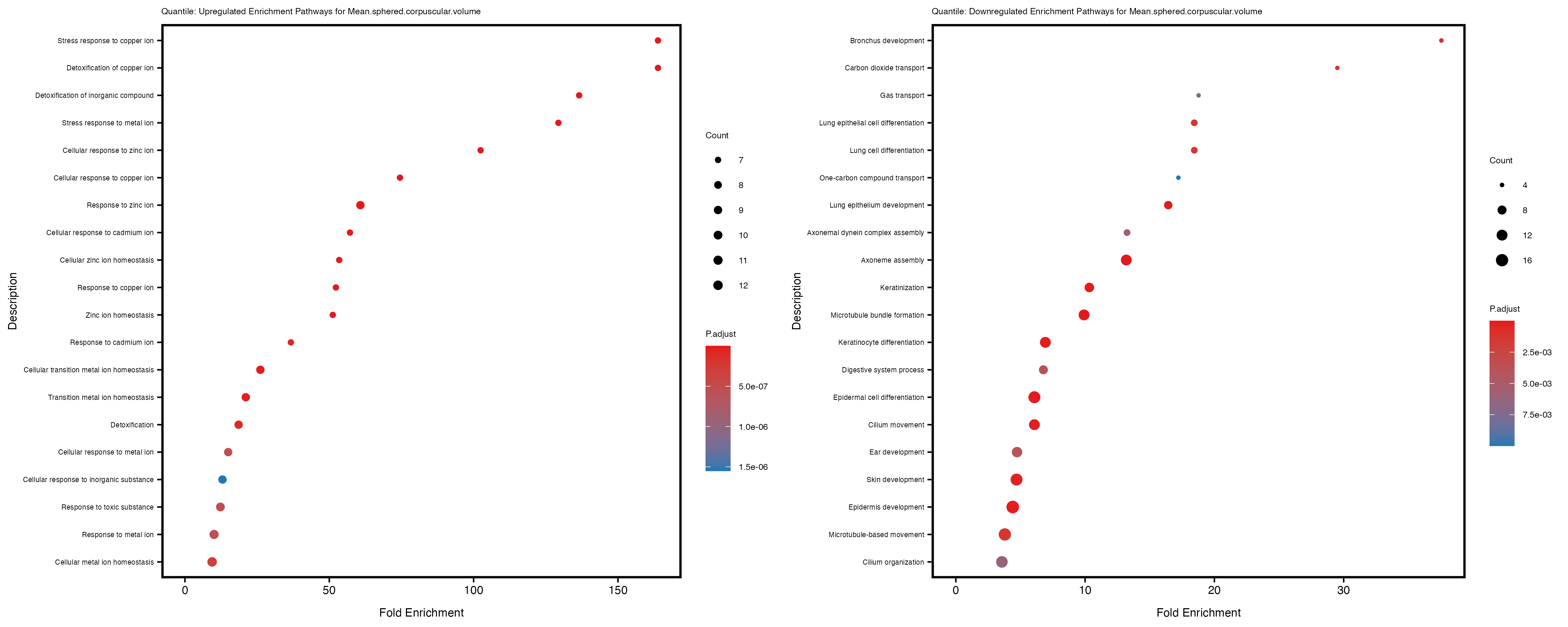
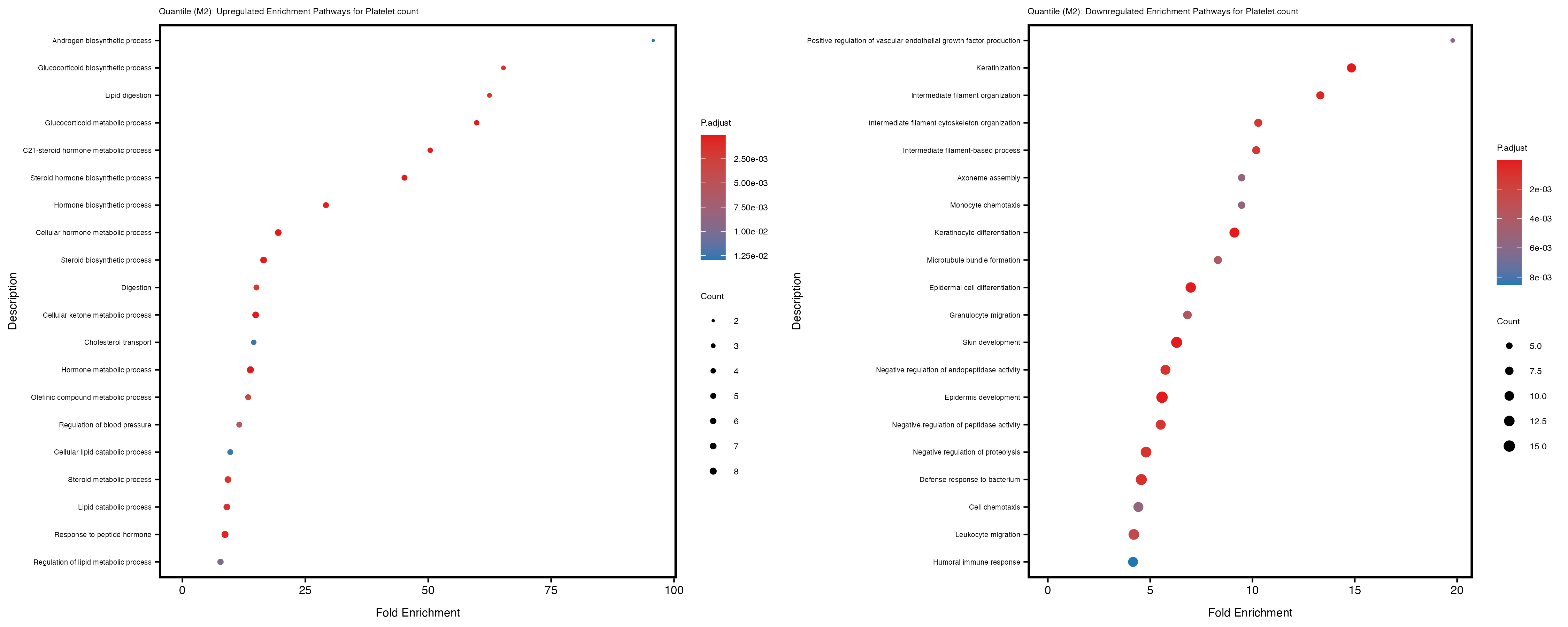
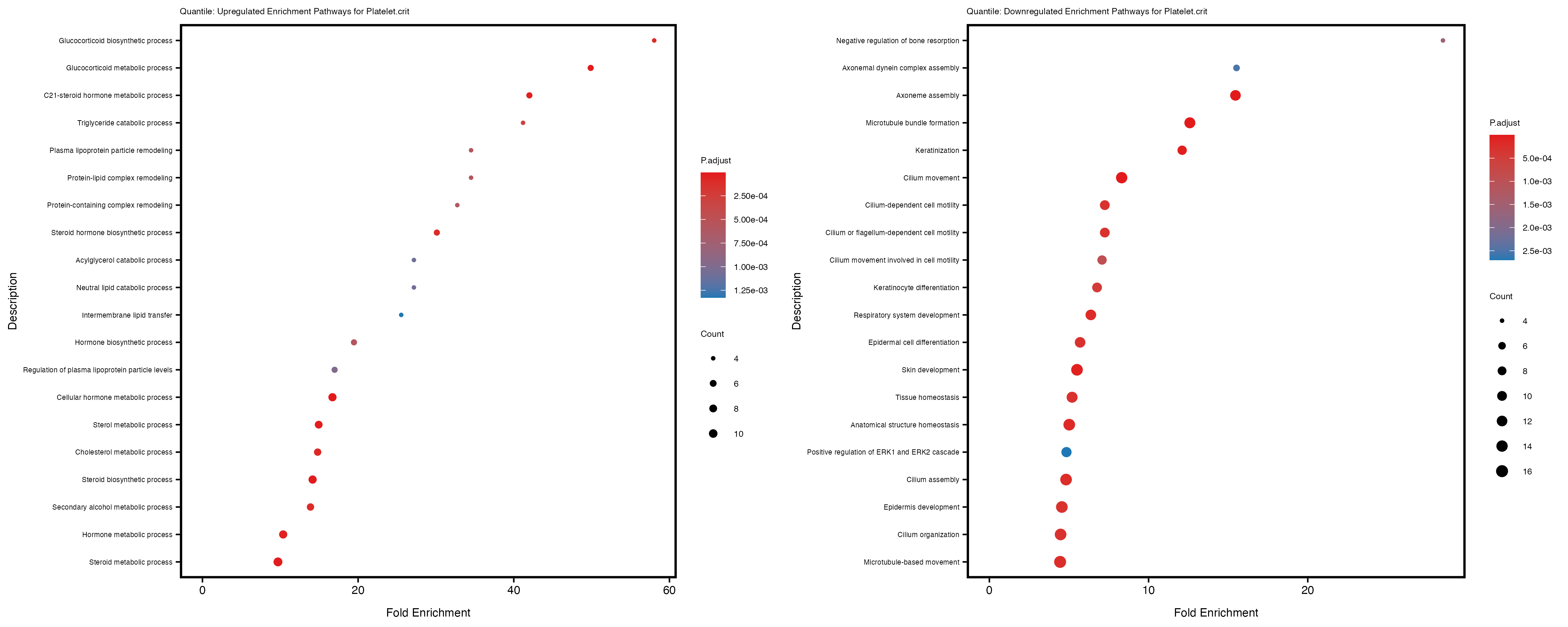
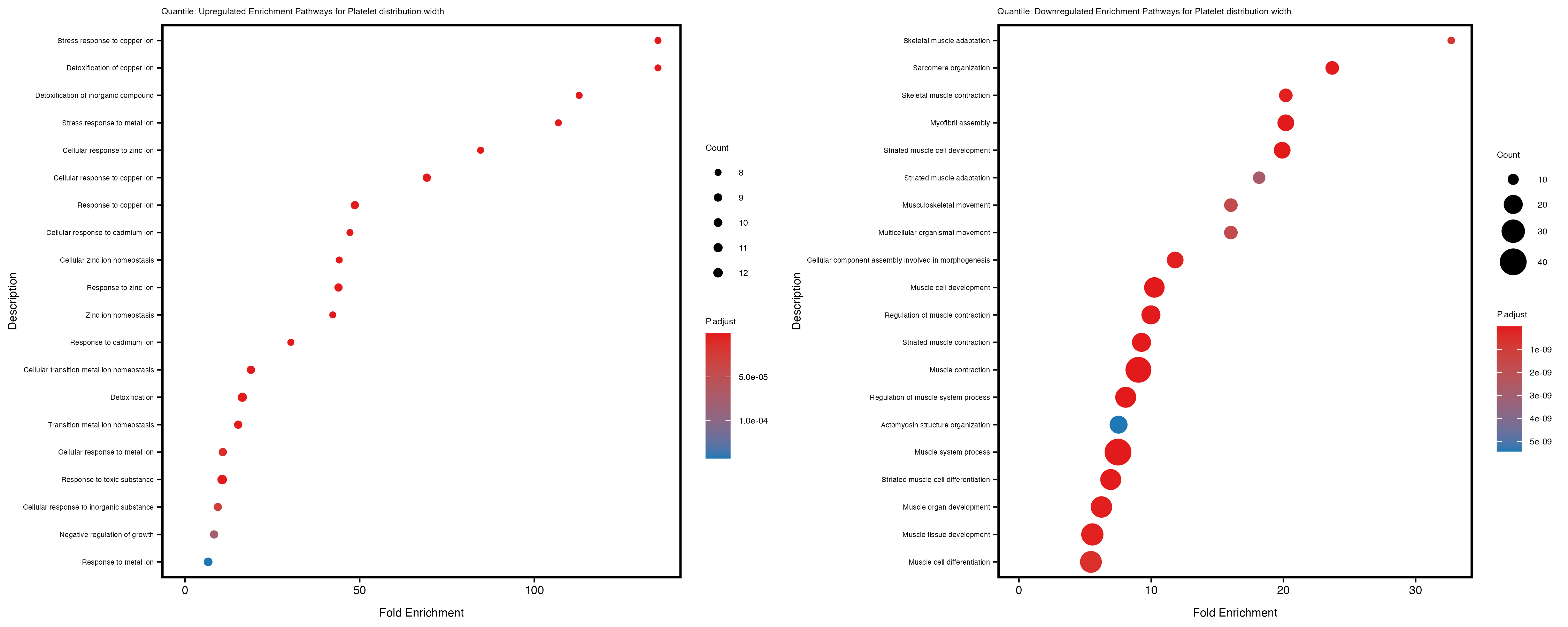
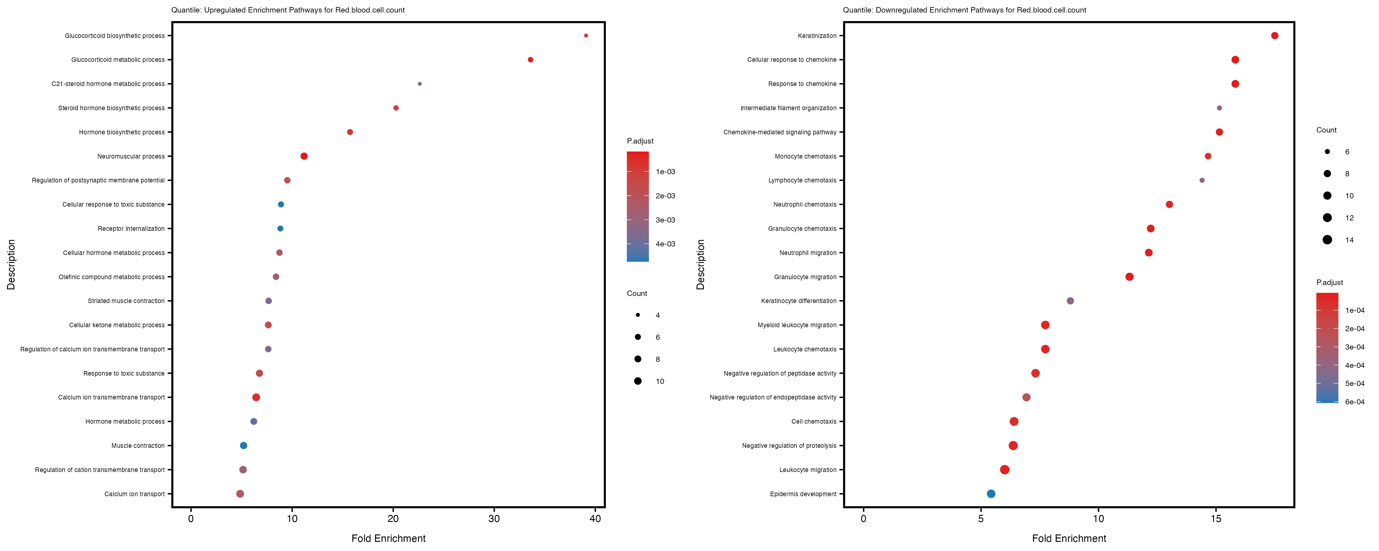
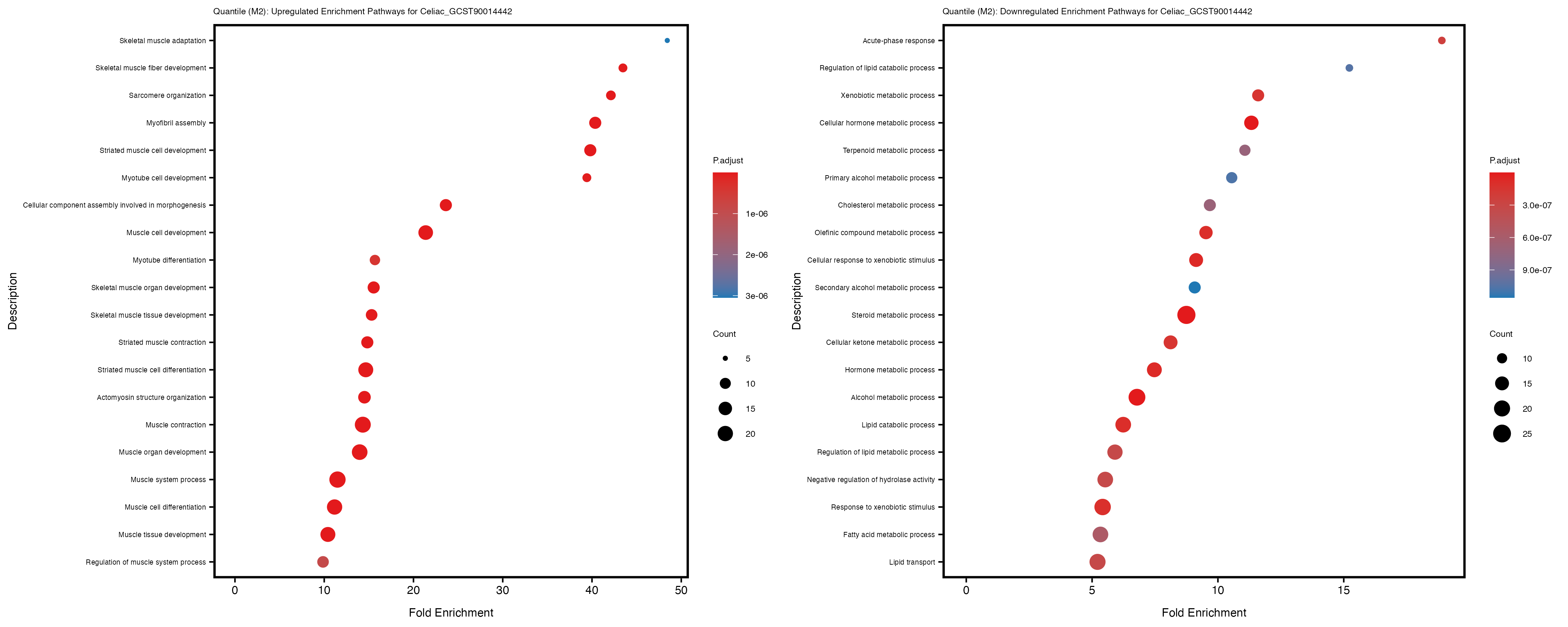
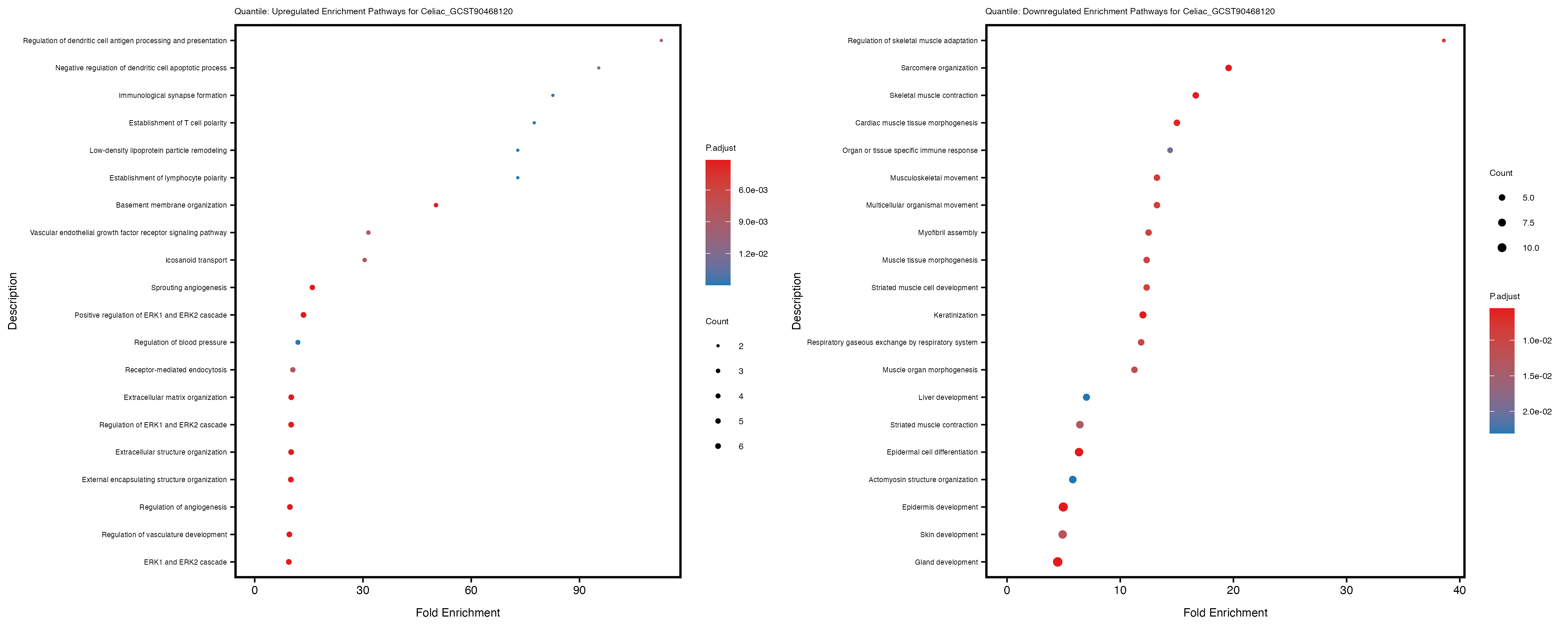
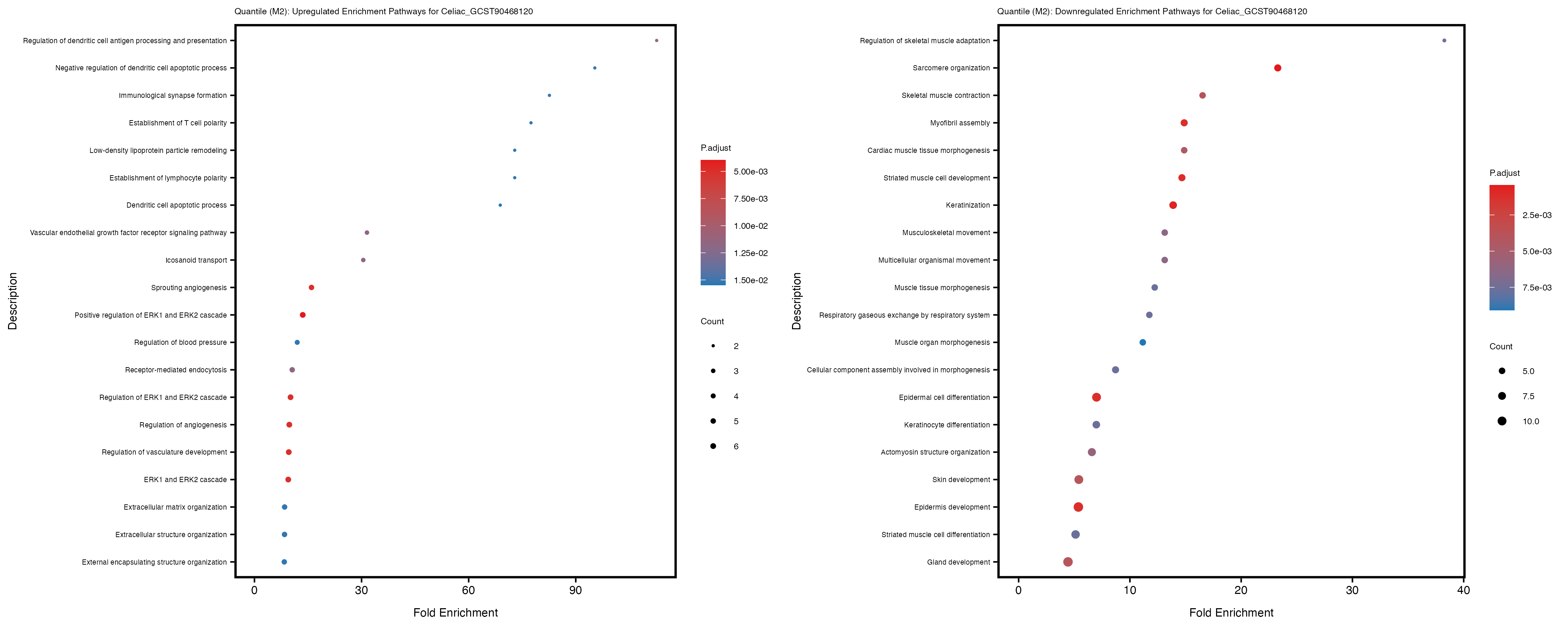
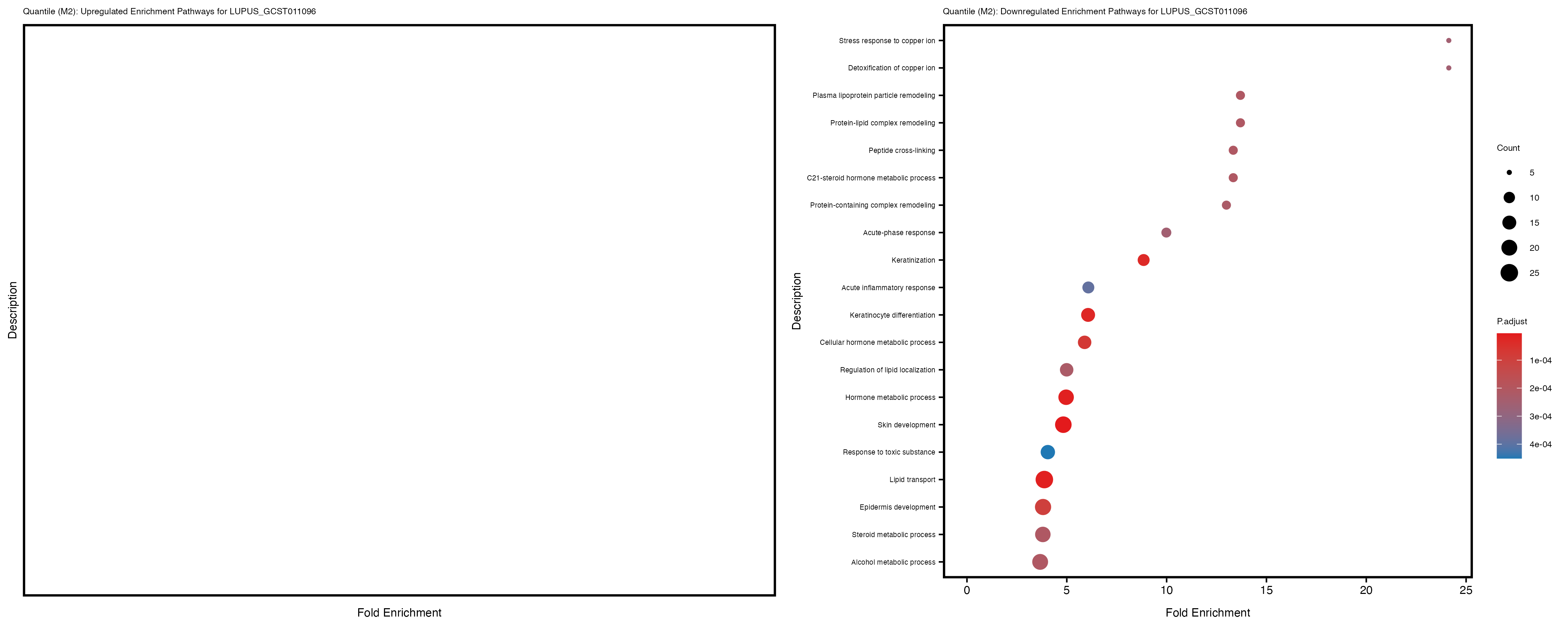
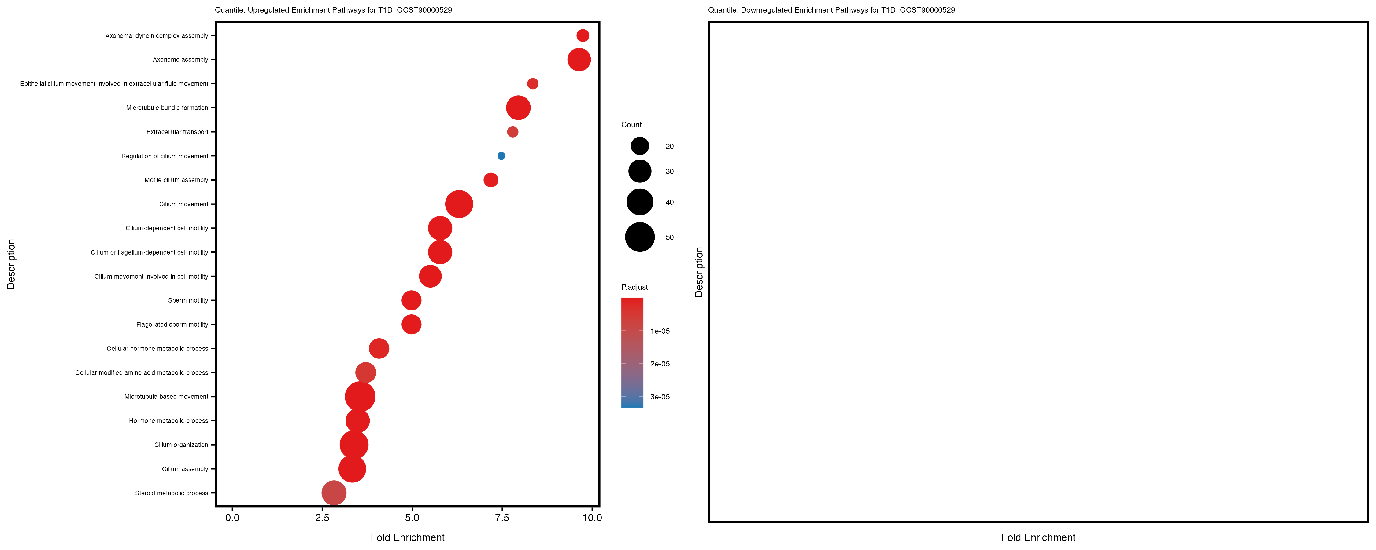
    labs(title = paste("Quantile: Upregulated Enrichment Pathways for", trait)) +
    theme(plot.title = element_text(size = 6), axis.text.y   = element_text(size = 5))
} else {
  enrich_plot_up <- plotEnrich(gse_up, plot_type = "dot", scale_ratio = 0.4) +
    labs(title = paste("Quantile: Upregulated Enrichment Pathways for", trait)) +
    theme(plot.title = element_text(size = 6), axis.text.y   = element_text(size = 5))
}
  
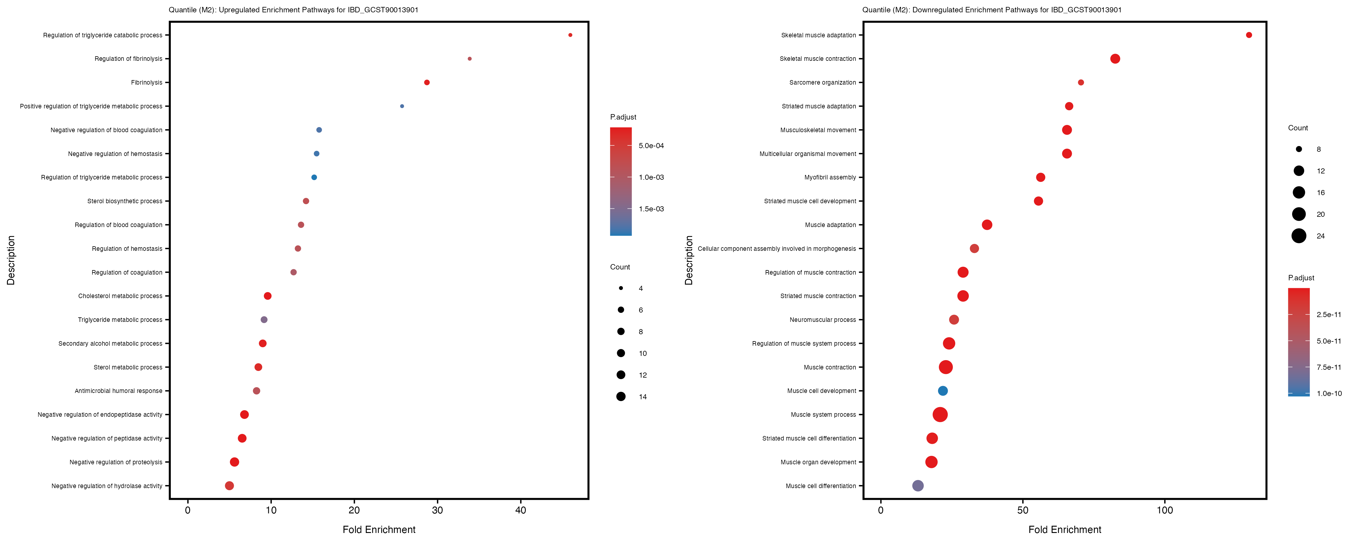
if (nrow(gse_down) >= 20) {
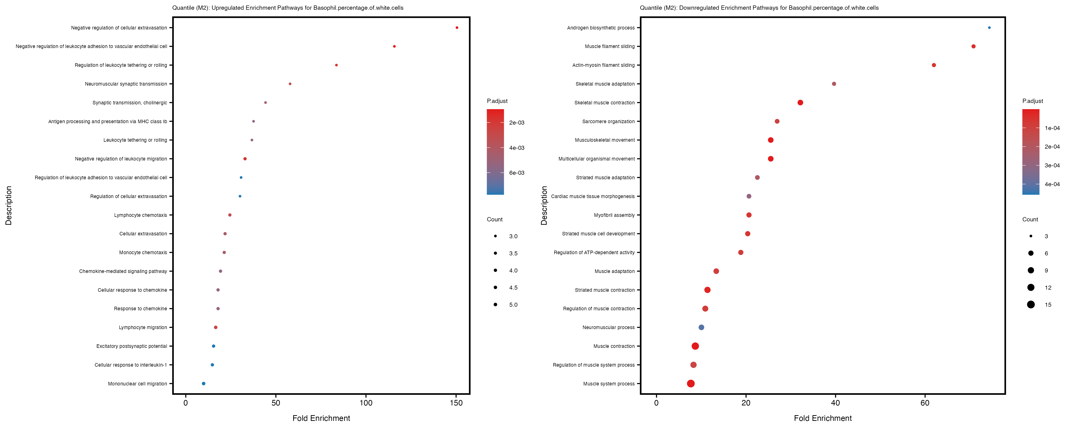
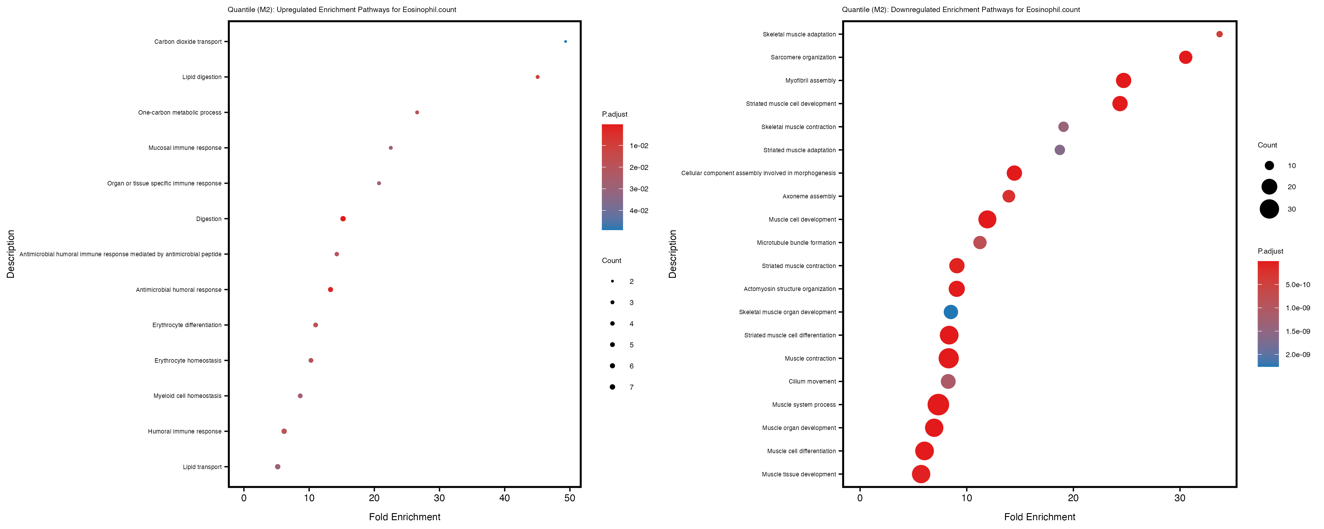
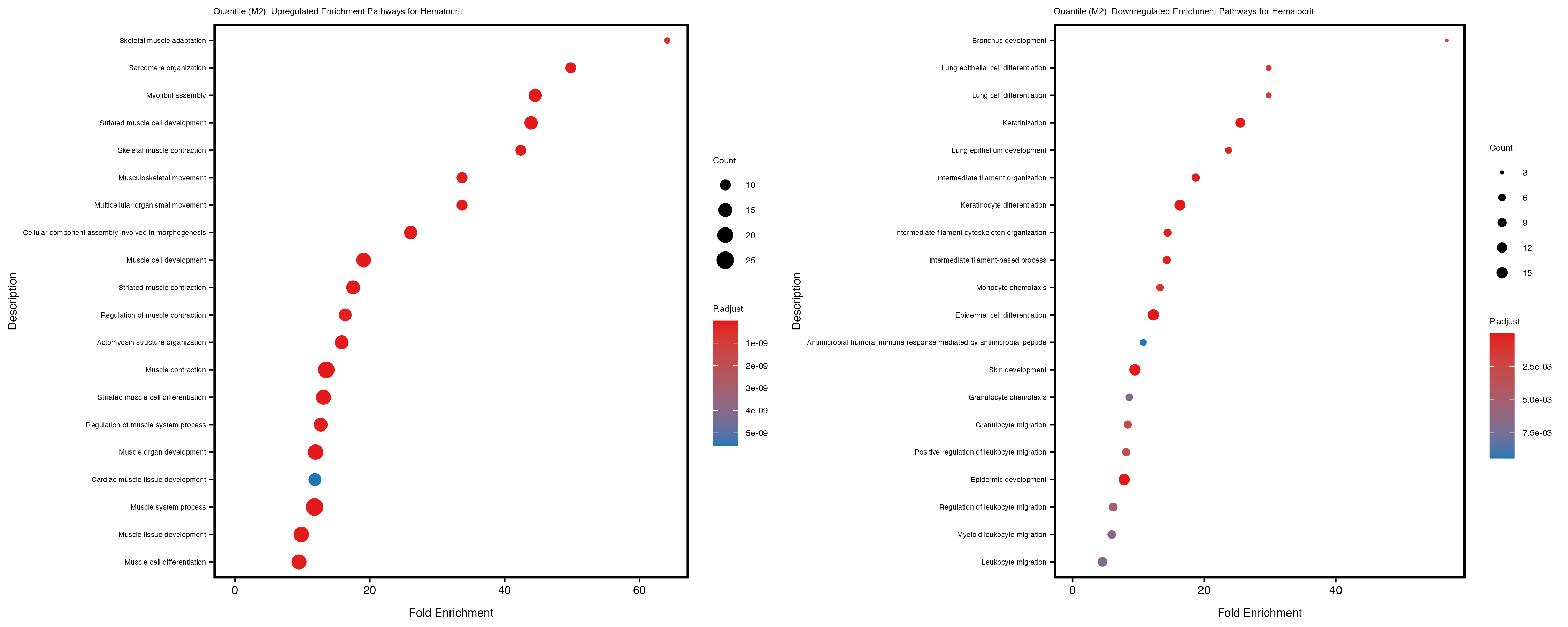
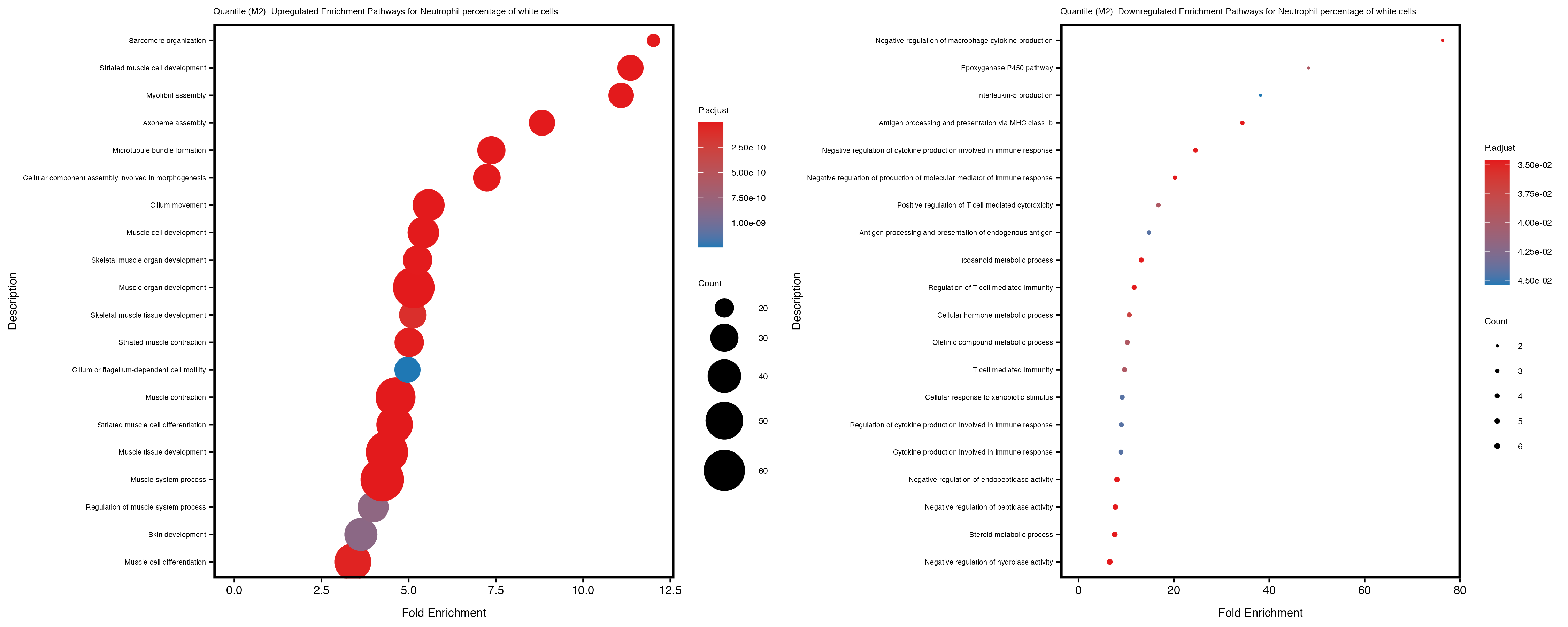
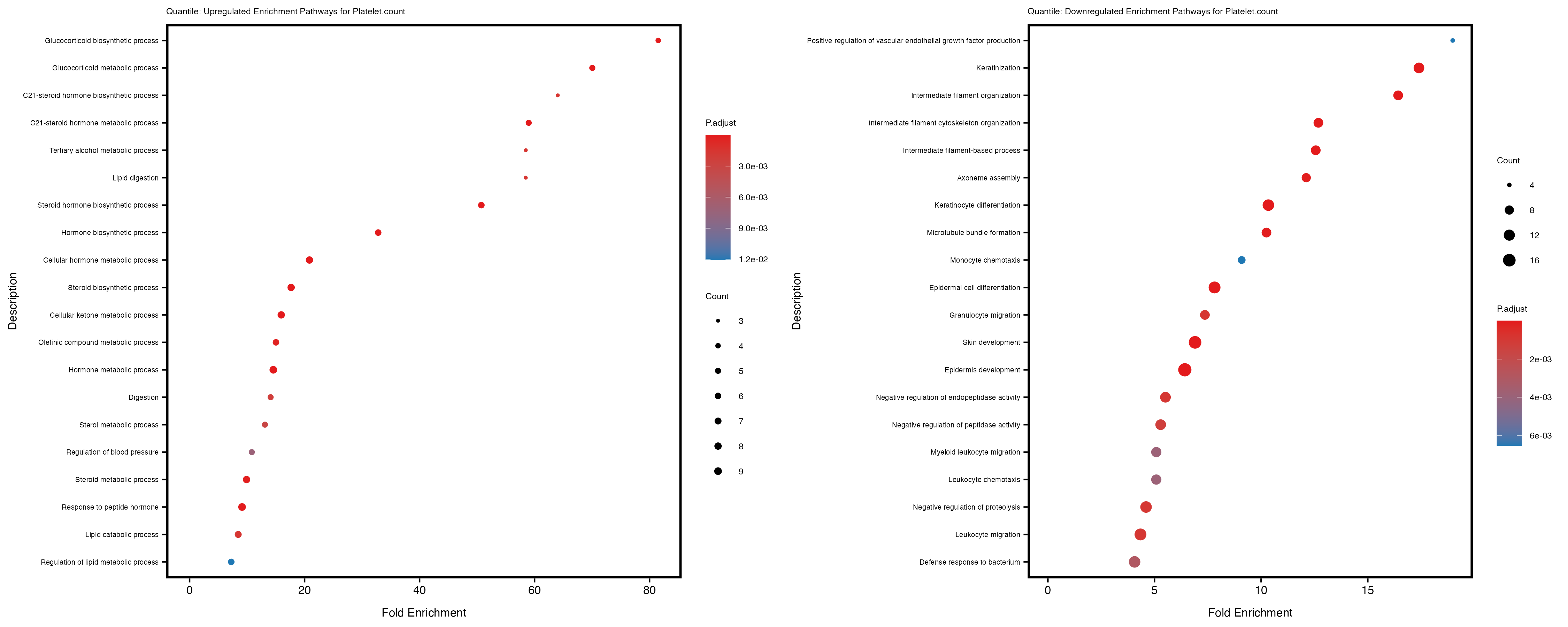
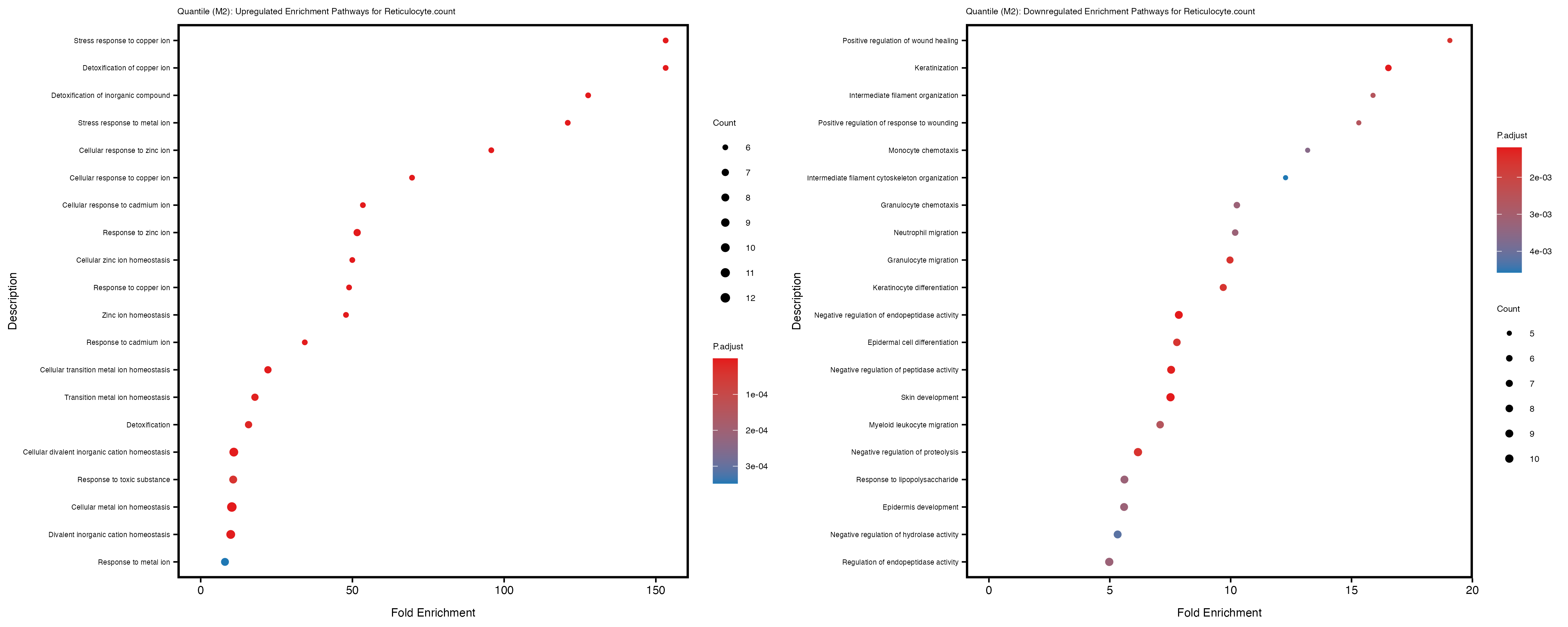
  enrich_plot_down <- plotEnrich(gse_down[1:20, ], plot_type = "dot", scale_ratio = 0.4) +
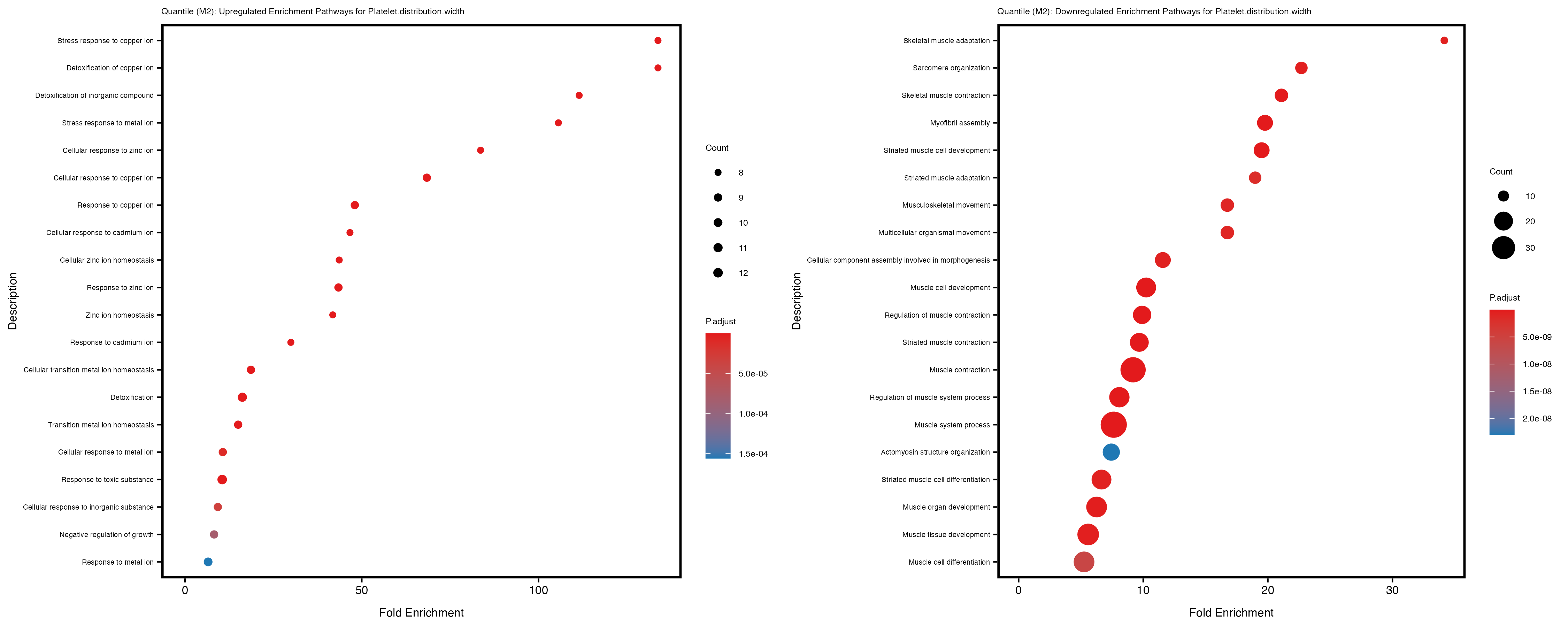
    labs(title = paste("Quantile: Downregulated Enrichment Pathways for", trait)) +
    theme(plot.title = element_text(size = 6), axis.text.y   = element_text(size = 5))
} else {
  enrich_plot_down <- plotEnrich(gse_down, plot_type = "dot", scale_ratio = 0.4) +
    labs(title = paste("Quantile: Downregulated Enrichment Pathways for", trait)) +
    theme(plot.title = element_text(size = 6), axis.text.y   = element_text(size = 5))
}
  
  # Arrange the two plots side by side
  combined_plot <- grid.arrange(enrich_plot_up, enrich_plot_down, ncol = 2)
  
  # Save the combined plot
  ggsave(paste0("enrichment_plot_quantile_", trait, ".png"), plot = combined_plot, 
         width = 15, height = 6)
  
  # Save the GO enrichment results to CSV
  write.csv(gse_up, file = paste0("GO_enrichment_", trait, "_quantile_upregulated.csv"))
  write.csv(gse_down, file = paste0("GO_enrichment_", trait, "_quantile_downregulated.csv"))
}

Result

Summary table

Continuous PRS without adjusting genotype PCs
Trait	Significant DE genes	Up-regulated Genes	Down-regulated Genes	Up-regulated GO pathways	Down-regulated GO pathways
Basophil.count	402	363	39	0	27
Basophil.percentage.of.white.cells	200	89	111	0	167
Celiac_GCST90014442	97	55	42	7	73
Celiac_GCST90468120	493	25	468	27	8
Eosinophil.count	338	128	210	0	88
Eosinophil.percentage.of.white.cells	209	85	124	1	28
Hematocrit	337	57	280	8	0
Hemoglobin.concentration	132	57	75	194	5
High.light.scatter.reticulocyte.count	239	52	187	34	73
High.light.scatter.reticulocyte.percentage.of.red.cells	325	94	231	15	161
IBD_GCST90013901	559	522	37	5	96
IBD_GCST90013951	380	338	42	199	71
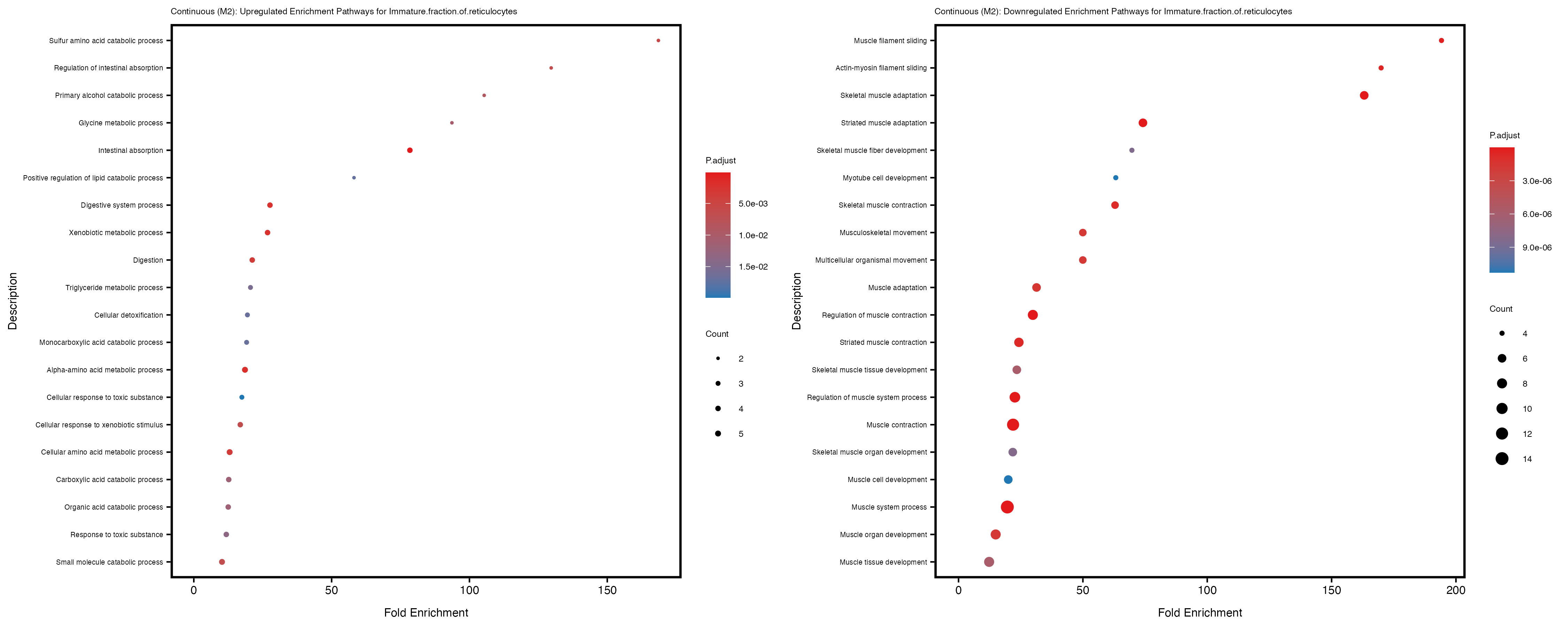
Immature.fraction.of.reticulocytes	288	134	154	43	73
LUPUS_GCST003156	119	79	40	48	39
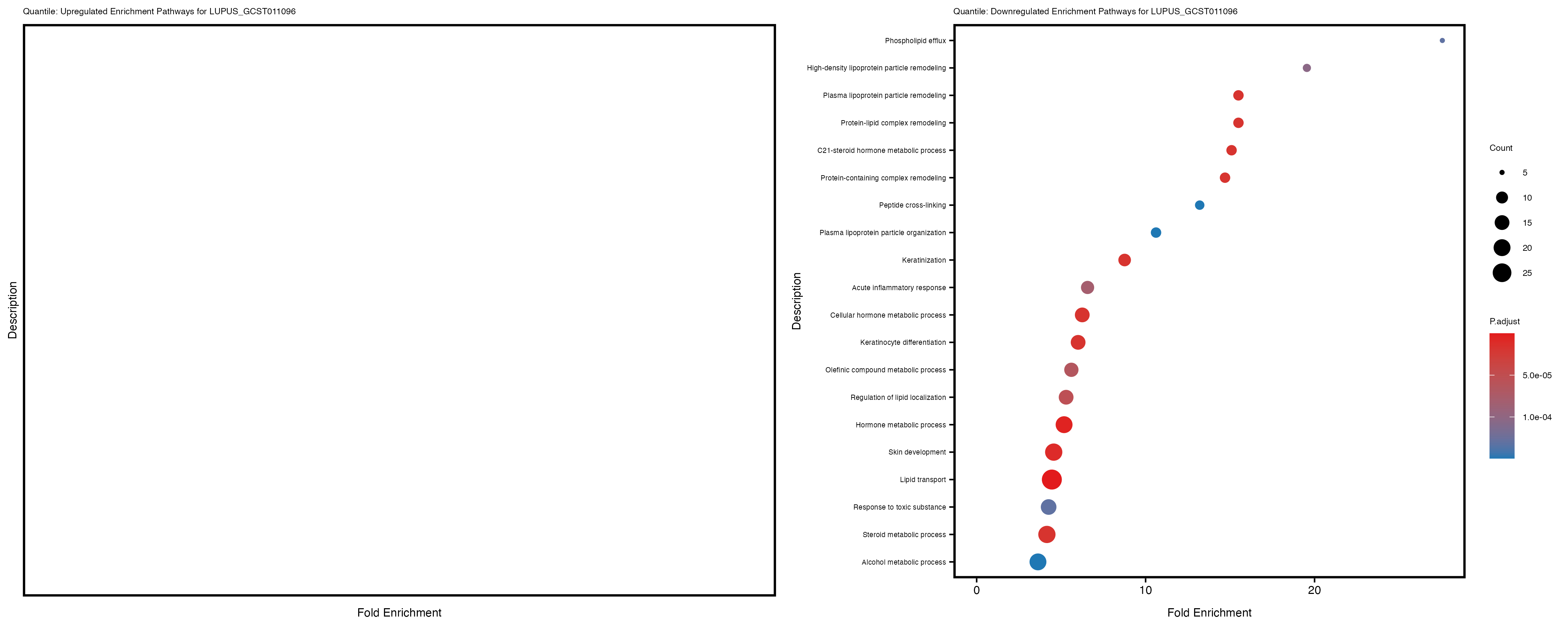
LUPUS_GCST011096	131	89	42	66	132
Lymphocyte.count	729	347	382	12	71
Lymphocyte.percentage.of.white.cells	927	305	622	3	33
Mean.corpuscular.hemoglobin	402	22	380	0	55
Mean.corpuscular.hemoglobin.concentration	788	69	719	20	193
Mean.corpuscular.volume	162	22	140	0	44
Mean.platelet.volume	146	30	116	39	7
Mean.reticulocyte.volume	312	148	164	110	4
Mean.sphered.corpuscular.volume	533	81	452	89	0
Monocyte.count	348	180	168	4	33
Monocyte.percentage.of.white.cells	179	42	137	55	13
Neutrophil.count	1358	1260	98	46	43
Neutrophil.percentage.of.white.cells	421	357	64	21	50
Platelet.count	78	51	27	0	8
Platelet.crit	113	82	31	13	0
Platelet.distribution.width	105	32	73	38	0
Red.blood.cell.count	130	81	49	56	0
Red.cell.distribution.width	999	396	603	77	18
Reticulocyte.count	140	60	80	2	164
Reticulocyte.fraction.of.red.cells	225	122	103	23	25
T1D_GCST90000529	618	540	78	30	22
T1D_GCST90014023	205	135	70	1	4
White.blood.cell.count	1314	1118	196	40	0

Continuous PRS with adjusting genotype PCs
Trait	Significant DE genes	Up-regulated Genes	Down-regulated Genes	Up-regulated GO pathways	Down-regulated GO pathways
Basophil.count	385	345	40	0	47
Basophil.percentage.of.white.cells	203	93	110	0	167
Celiac_GCST90014442	94	55	39	2	114
Celiac_GCST90468120	493	25	468	2	9
Eosinophil.count	333	126	207	0	89
Eosinophil.percentage.of.white.cells	211	87	124	1	21
Hematocrit	318	51	267	8	0
Hemoglobin.concentration	120	54	66	0	0
High.light.scatter.reticulocyte.count	237	52	185	34	74
High.light.scatter.reticulocyte.percentage.of.red.cells	328	101	227	14	153
IBD_GCST90013901	561	525	36	15	96
IBD_GCST90013951	378	340	38	183	71
Immature.fraction.of.reticulocytes	294	142	152	44	73
LUPUS_GCST003156	123	82	41	42	279
LUPUS_GCST011096	138	94	44	60	236
Lymphocyte.count	718	341	377	8	74
Lymphocyte.percentage.of.white.cells	923	309	614	3	30
Mean.corpuscular.hemoglobin	381	22	359	0	63
Mean.corpuscular.hemoglobin.concentration	785	71	714	0	244
Mean.corpuscular.volume	162	22	140	0	40
Mean.platelet.volume	147	31	116	5	9
Mean.reticulocyte.volume	312	147	165	105	2
Mean.sphered.corpuscular.volume	534	84	450	43	0
Monocyte.count	366	188	178	10	33
Monocyte.percentage.of.white.cells	182	43	139	30	21
Neutrophil.count	1374	1271	103	44	43
Neutrophil.percentage.of.white.cells	428	361	67	19	18
Platelet.count	73	47	26	0	8
Platelet.crit	110	80	30	13	0
Platelet.distribution.width	93	31	62	39	0
Red.blood.cell.count	110	67	43	29	0
Red.cell.distribution.width	990	401	589	16	19
Reticulocyte.count	129	57	72	2	150
Reticulocyte.fraction.of.red.cells	213	120	93	23	0
T1D_GCST90000529	619	537	82	32	23
T1D_GCST90014023	192	123	69	2	4
White.blood.cell.count	1313	1118	195	39	48

Quantile PRS without adjusting genotype PCs
Trait	Significant DE genes	Up-regulated Genes	Down-regulated Genes	Up-regulated GO pathways	Down-regulated GO pathways
Basophil.count_quantile	712	685	27	144	16
Basophil.percentage.of.white.cells_quantile	184	64	120	61	89
Celiac_GCST90014442_quantile	336	124	212	105	320
Celiac_GCST90468120_quantile	212	42	170	94	27
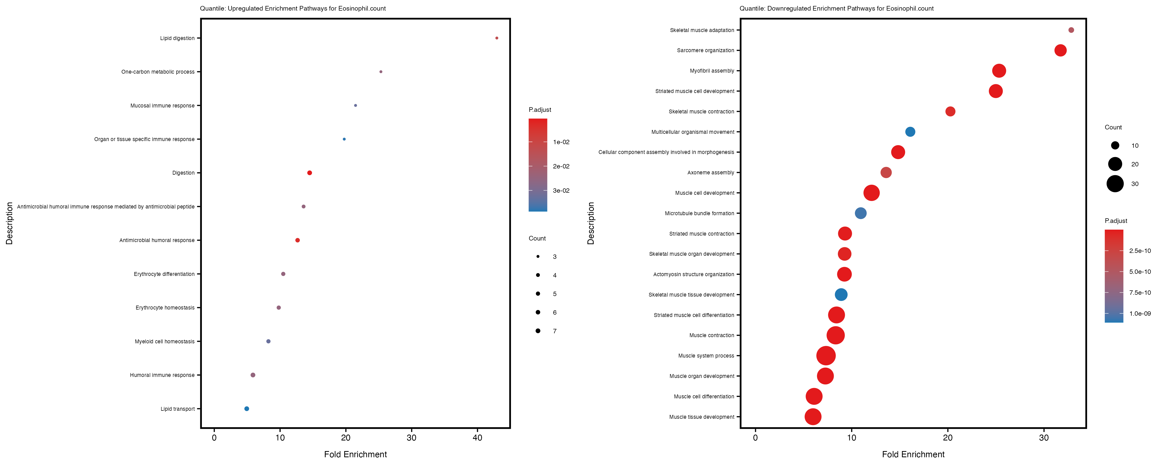
Eosinophil.count_quantile	507	197	310	12	157
Eosinophil.percentage.of.white.cells_quantile	431	218	213	3	165
Hematocrit_quantile	269	118	151	114	35
Hemoglobin.concentration_quantile	160	37	123	36	104
High.light.scatter.reticulocyte.count_quantile	225	93	132	61	98
High.light.scatter.reticulocyte.percentage.of.red.cells_quantile	312	141	171	49	158
IBD_GCST90013901_quantile	272	204	68	147	130
IBD_GCST90013951_quantile	346	256	90	158	65
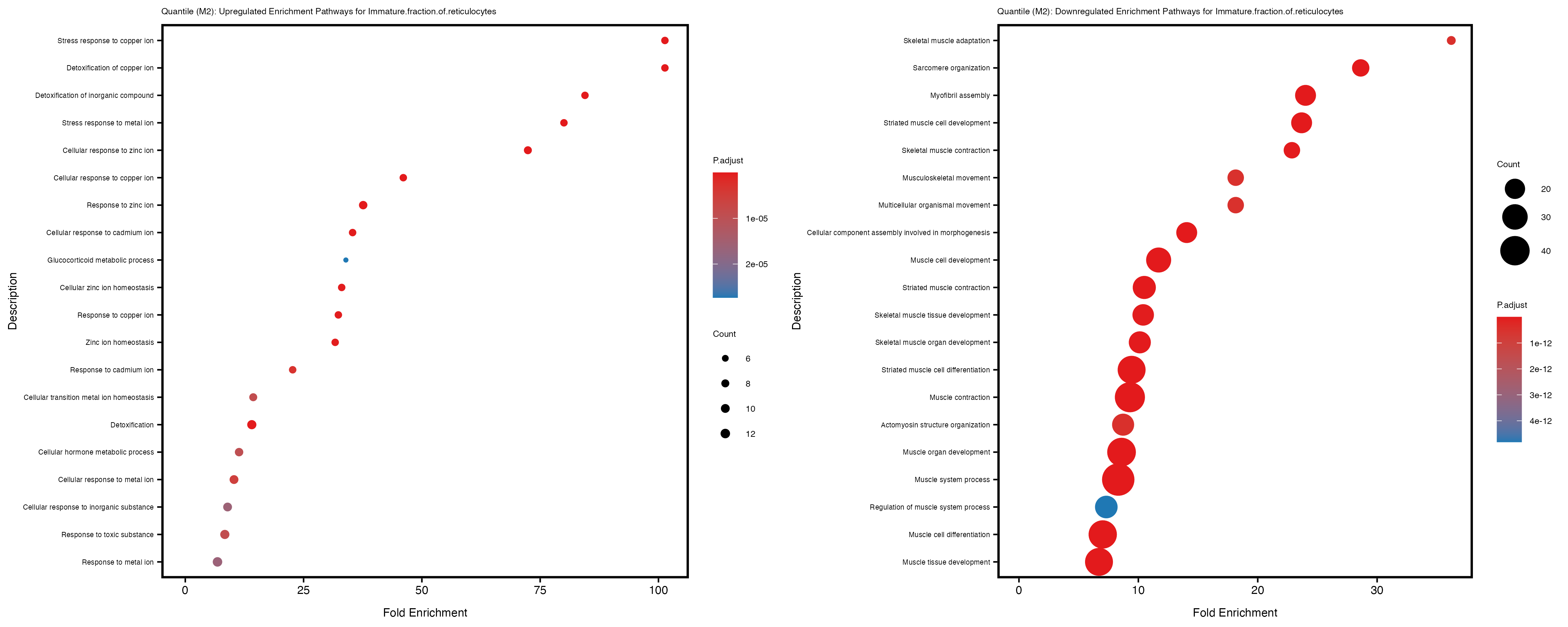
Immature.fraction.of.reticulocytes_quantile	473	128	345	104	149
LUPUS_GCST003156_quantile	205	96	109	20	57
LUPUS_GCST011096_quantile	493	52	441	0	202
Lymphocyte.count_quantile	1456	852	604	95	188
Lymphocyte.percentage.of.white.cells_quantile	532	289	243	37	112
Mean.corpuscular.hemoglobin_quantile	410	23	387	40	89
Mean.corpuscular.hemoglobin.concentration_quantile	317	86	231	30	336
Mean.corpuscular.volume_quantile	453	58	395	119	98
Mean.platelet.volume_quantile	209	85	124	55	26
Mean.reticulocyte.volume_quantile	406	115	291	106	45
Mean.sphered.corpuscular.volume_quantile	355	76	279	55	48
Monocyte.count_quantile	1175	845	330	109	62
Monocyte.percentage.of.white.cells_quantile	566	50	516	36	69
Neutrophil.count_quantile	806	736	70	105	13
Neutrophil.percentage.of.white.cells_quantile	1451	1330	121	396	31
Platelet.count_quantile	248	59	189	59	48
Platelet.crit_quantile	314	100	214	59	103
Platelet.distribution.width_quantile	469	149	320	39	160
Red.blood.cell.count_quantile	291	157	134	103	61
Red.cell.distribution.width_quantile	399	287	112	45	24
Reticulocyte.count_quantile	170	74	96	34	68
Reticulocyte.fraction.of.red.cells_quantile	517	458	59	191	1
T1D_GCST90000529_quantile	1559	1438	121	268	0
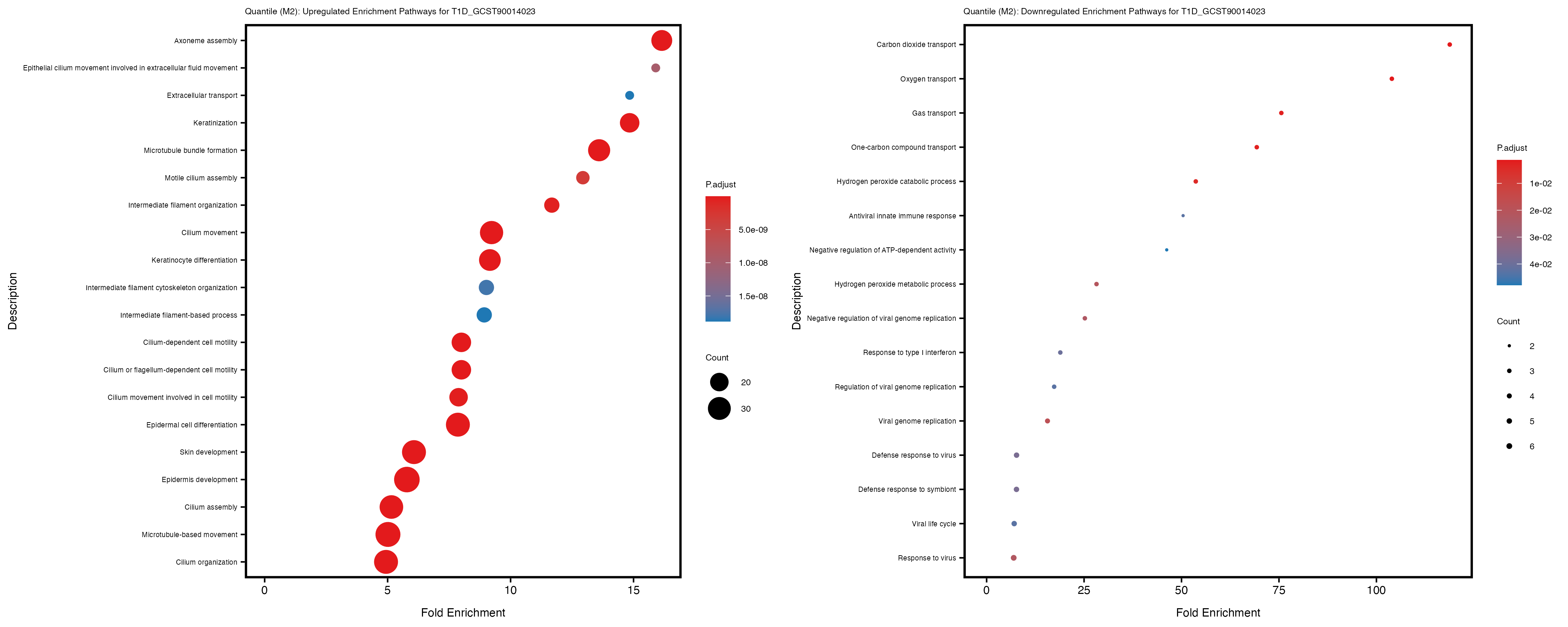
T1D_GCST90014023_quantile	575	504	71	87	18
White.blood.cell.count_quantile	1216	1082	134	156	118

Quantile PRS with adjusting genotype PCs
Trait	Significant DE genes	Up-regulated Genes	Down-regulated Genes	Up-regulated GO pathways	Down-regulated GO pathways
Basophil.count_quantile	707	682	25	148	32
Basophil.percentage.of.white.cells_quantile	174	62	112	70	89
Celiac_GCST90014442_quantile	335	124	211	106	306
Celiac_GCST90468120_quantile	208	43	165	86	28
Eosinophil.count_quantile	498	191	307	13	158
Eosinophil.percentage.of.white.cells_quantile	426	219	207	3	160
Hematocrit_quantile	235	108	127	114	37
Hemoglobin.concentration_quantile	156	35	121	0	117
High.light.scatter.reticulocyte.count_quantile	218	94	124	62	82
High.light.scatter.reticulocyte.percentage.of.red.cells_quantile	316	149	167	42	151
IBD_GCST90013901_quantile	269	200	69	142	129
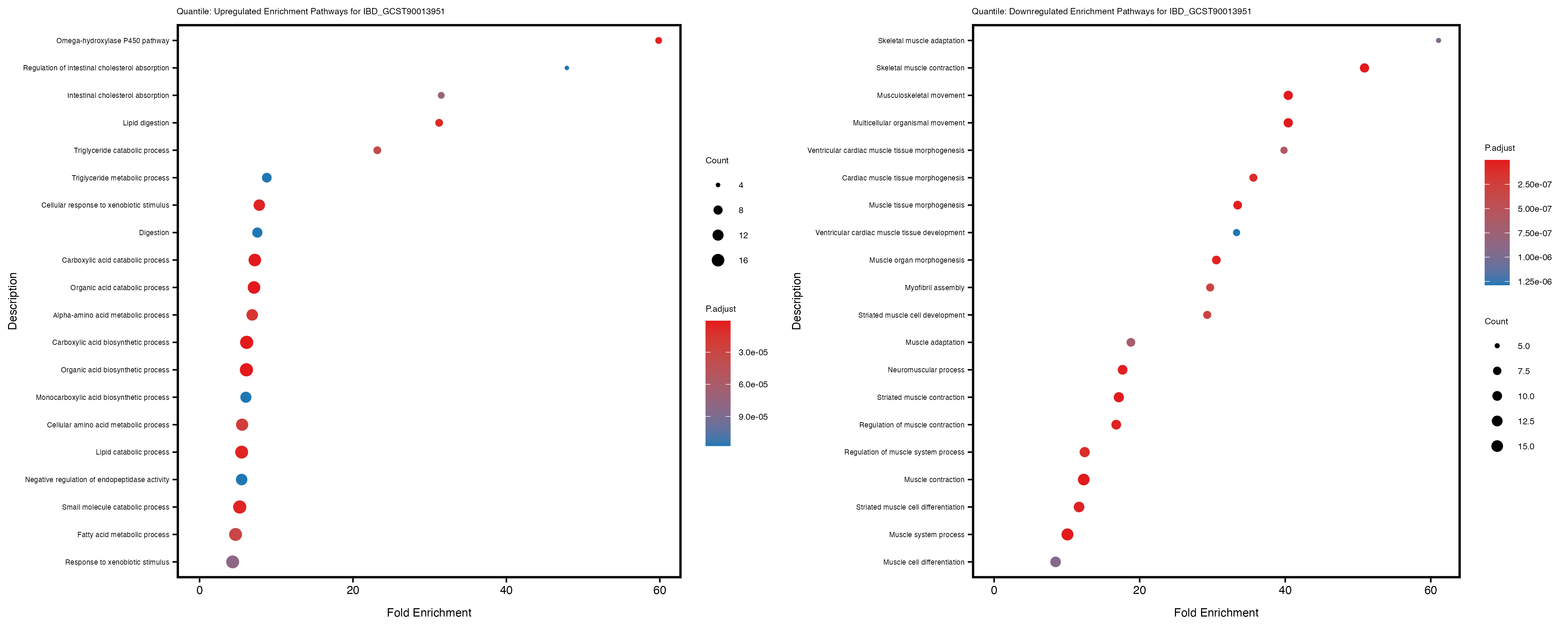
IBD_GCST90013951_quantile	337	250	87	168	66
Immature.fraction.of.reticulocytes_quantile	456	127	329	103	146
LUPUS_GCST003156_quantile	202	97	105	17	61
LUPUS_GCST011096_quantile	471	47	424	0	173
Lymphocyte.count_quantile	1603	907	696	109	228
Lymphocyte.percentage.of.white.cells_quantile	511	285	226	37	117
Mean.corpuscular.hemoglobin_quantile	390	25	365	41	100
Mean.corpuscular.hemoglobin.concentration_quantile	316	91	225	48	331
Mean.corpuscular.volume_quantile	425	55	370	110	106
Mean.platelet.volume_quantile	205	85	120	106	28
Mean.reticulocyte.volume_quantile	403	111	292	115	34
Mean.sphered.corpuscular.volume_quantile	366	78	288	62	45
Monocyte.count_quantile	1186	844	342	104	49
Monocyte.percentage.of.white.cells_quantile	589	50	539	18	82
Neutrophil.count_quantile	808	736	72	121	13
Neutrophil.percentage.of.white.cells_quantile	1467	1335	132	416	21
Platelet.count_quantile	235	53	182	49	61
Platelet.crit_quantile	309	93	216	68	92
Platelet.distribution.width_quantile	450	147	303	32	150
Red.blood.cell.count_quantile	264	143	121	116	81
Red.cell.distribution.width_quantile	405	293	112	44	23
Reticulocyte.count_quantile	169	74	95	36	66
Reticulocyte.fraction.of.red.cells_quantile	516	461	55	225	3
T1D_GCST90000529_quantile	1543	1417	126	243	0
T1D_GCST90014023_quantile	554	482	72	91	16
White.blood.cell.count_quantile	1173	1042	131	181	120

Interpretation:

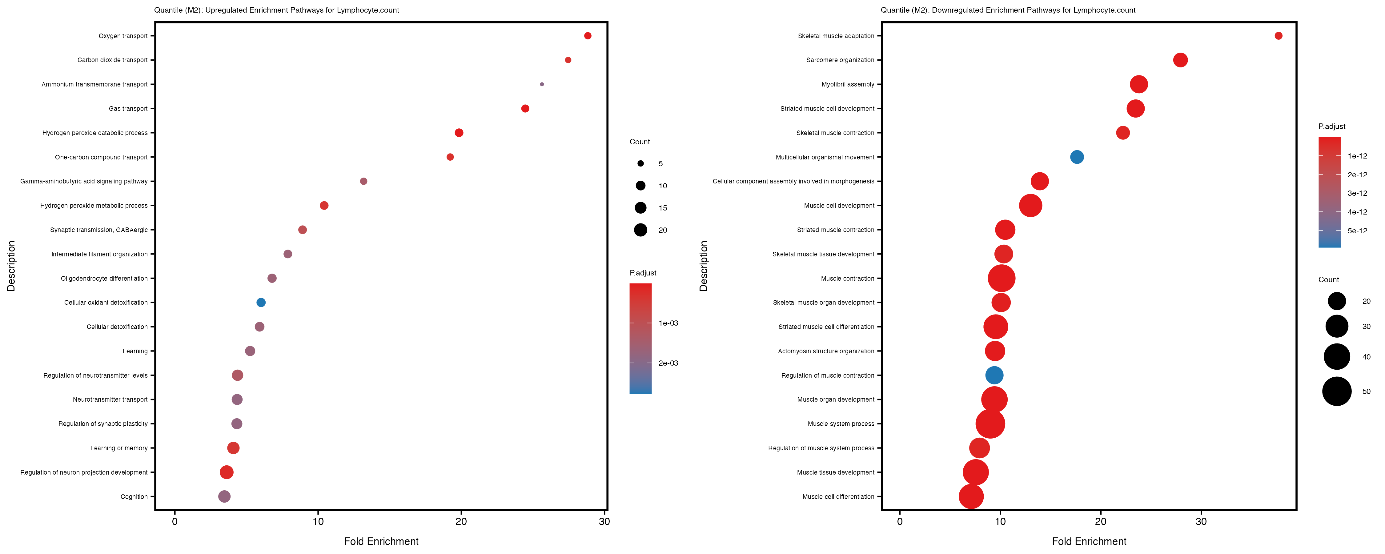
In the quantile analysis, the number of significant differential expressed genes is generally higher compared to the continuous analysis, which suggests that stratifying by PRS (top 25%) may identify more genes with stronger associations to the traits. We observed that certain genes were identified in both the continuous and quantile PRS analyses, though not all genes overlapped. Specifically, for the Eosinophil count trait, ACTN3, HAMP, SCGB3A1, CH25H, and NPIPA8 appeared among the top 10 DEGs across both analyses, suggesting that these genes might play a key role in the trait regardless of the analysis approach. For example:

HAMP encodes Hepcidin, which is involved in the maintenance of iron homeostasis.
SCGB3A1 predicts to enable cytokin activity.
CH25H encodes for cholesterol 25-hydroxylase, involved in lipid metabolism and modulating immune responses.

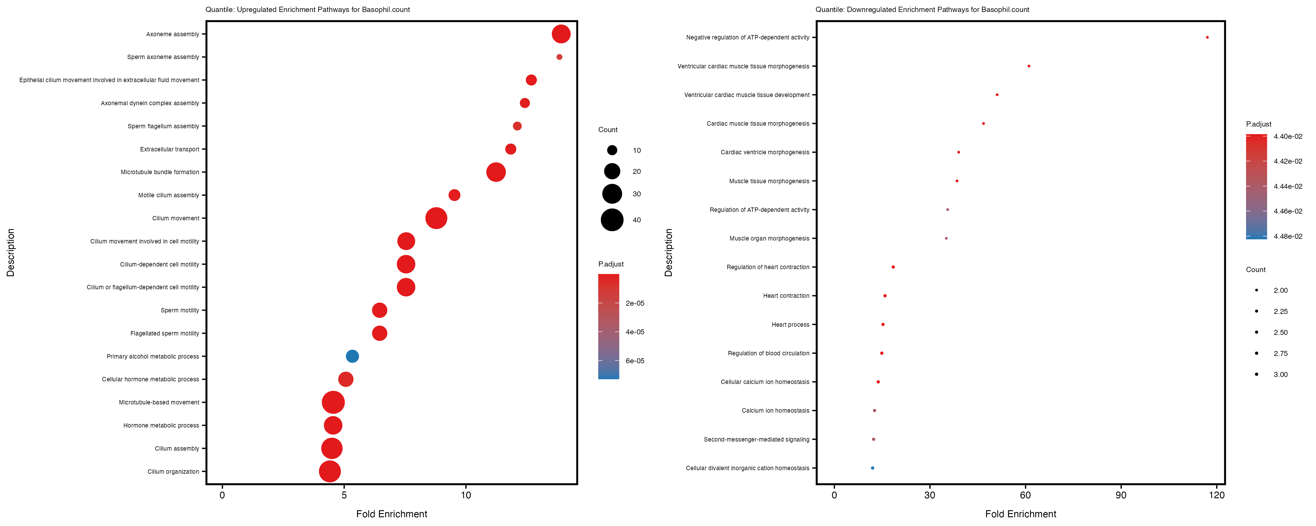
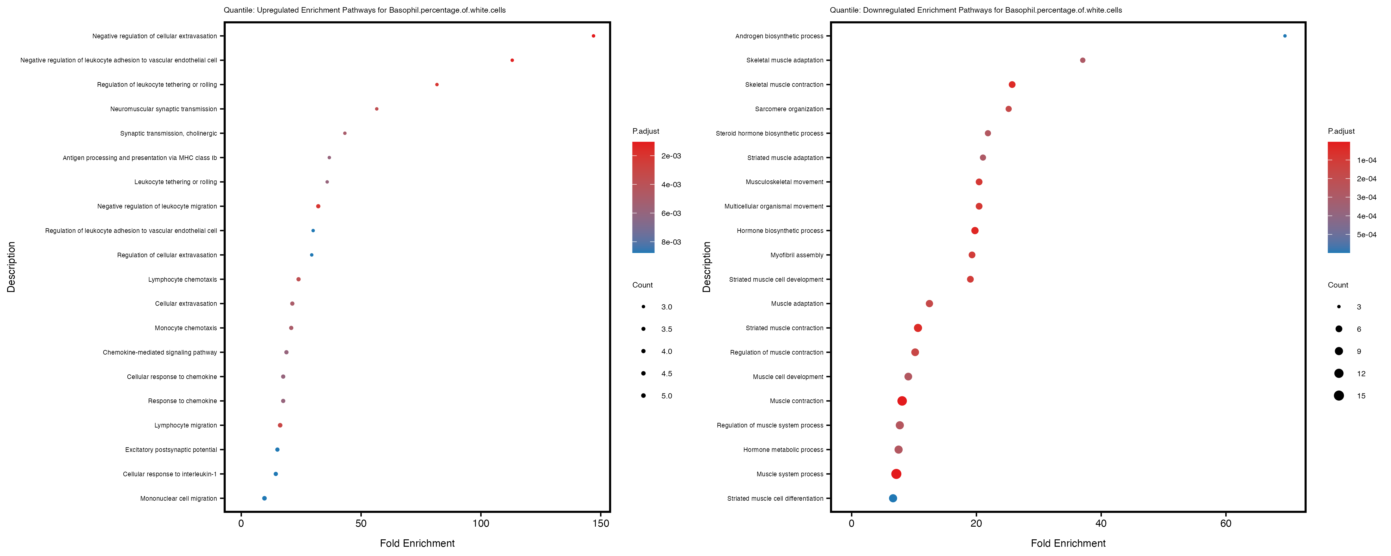
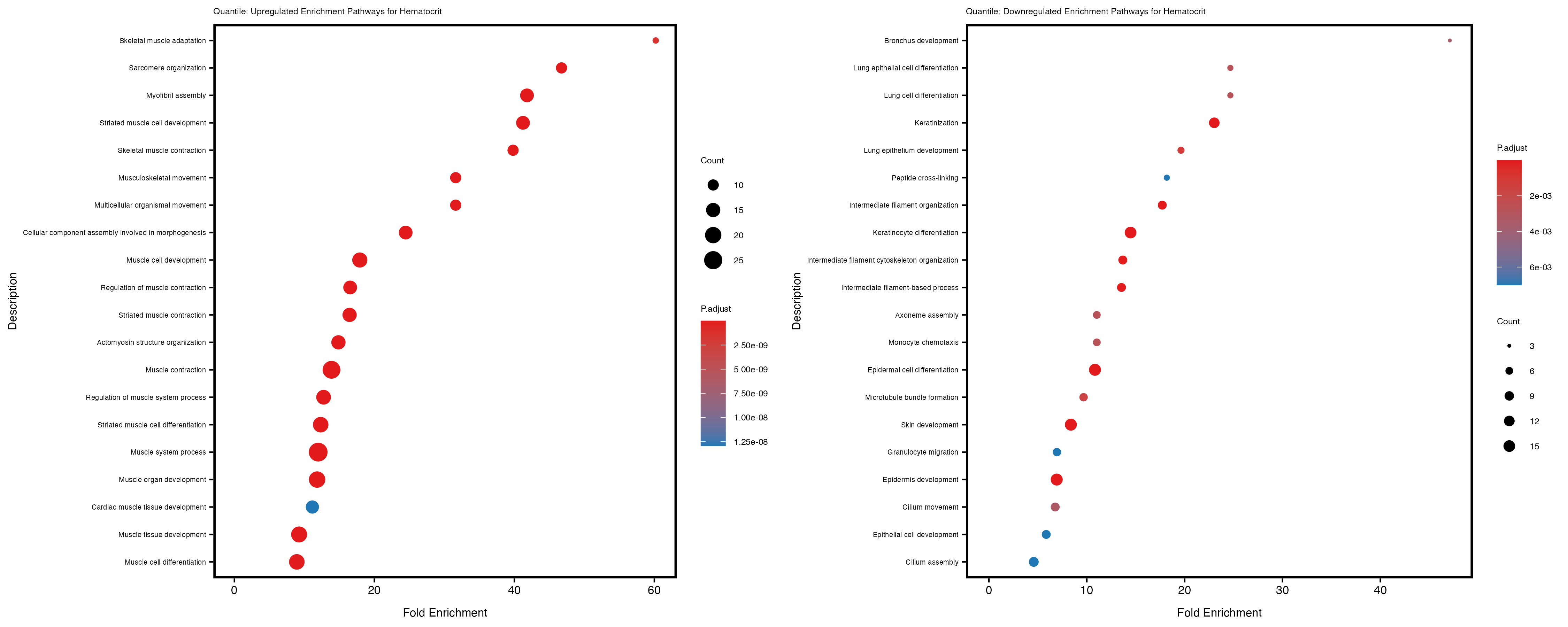
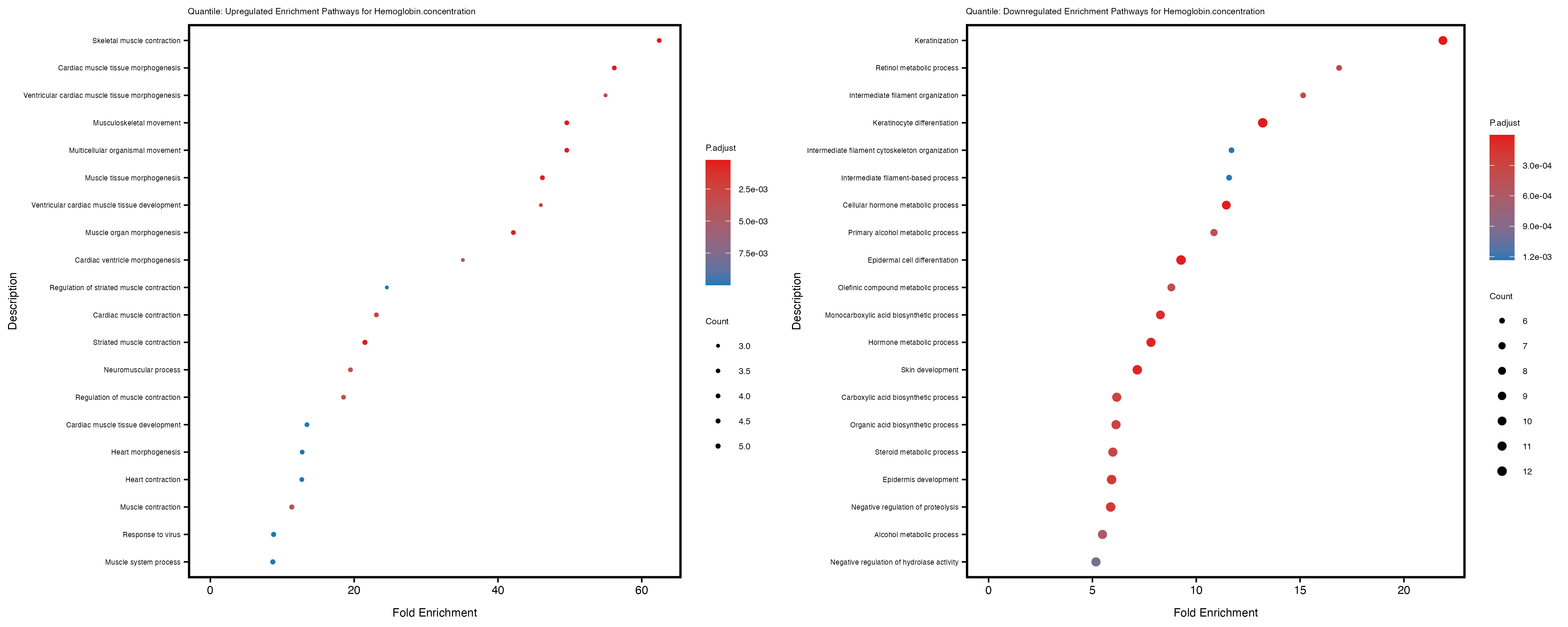
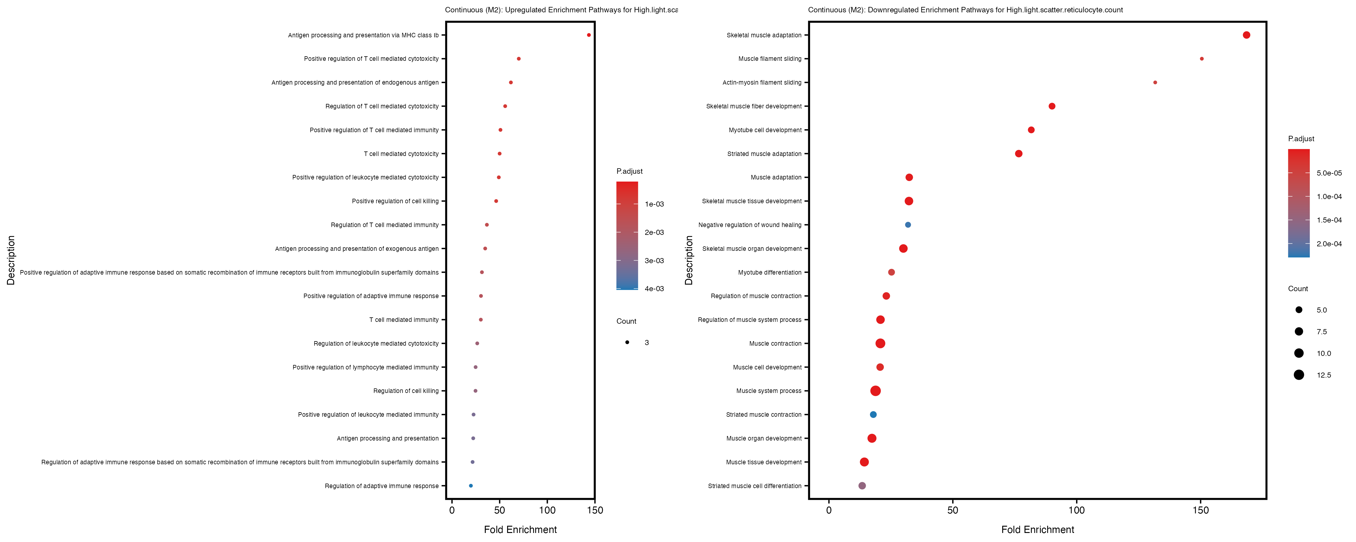
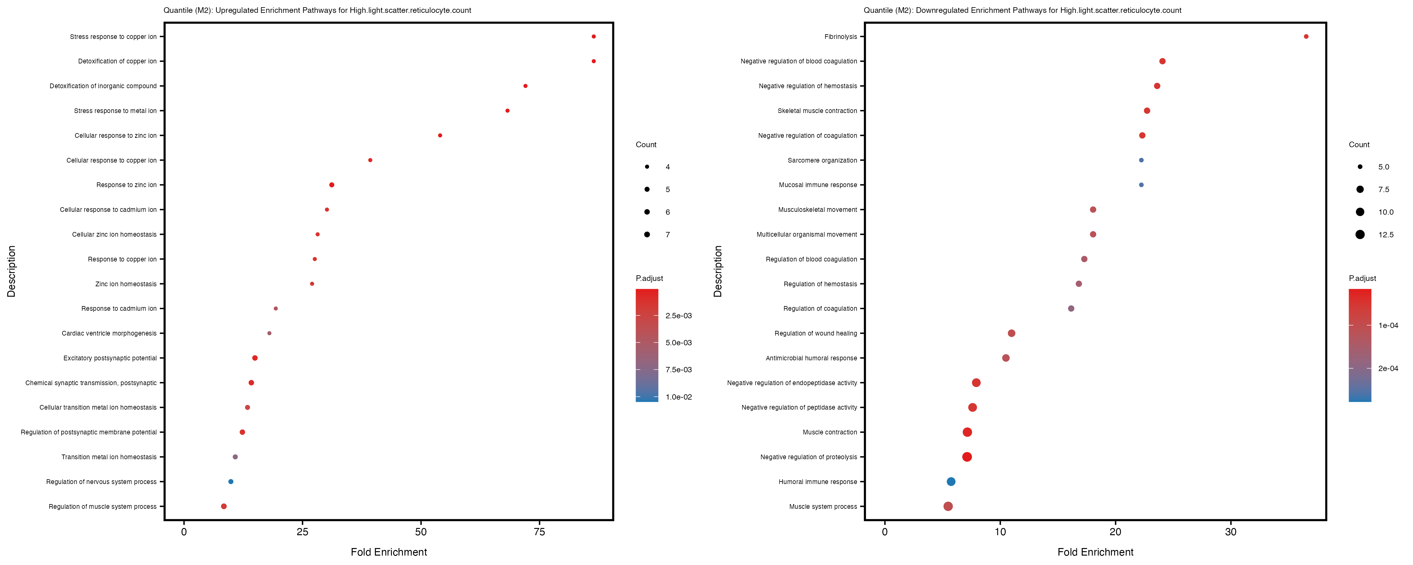
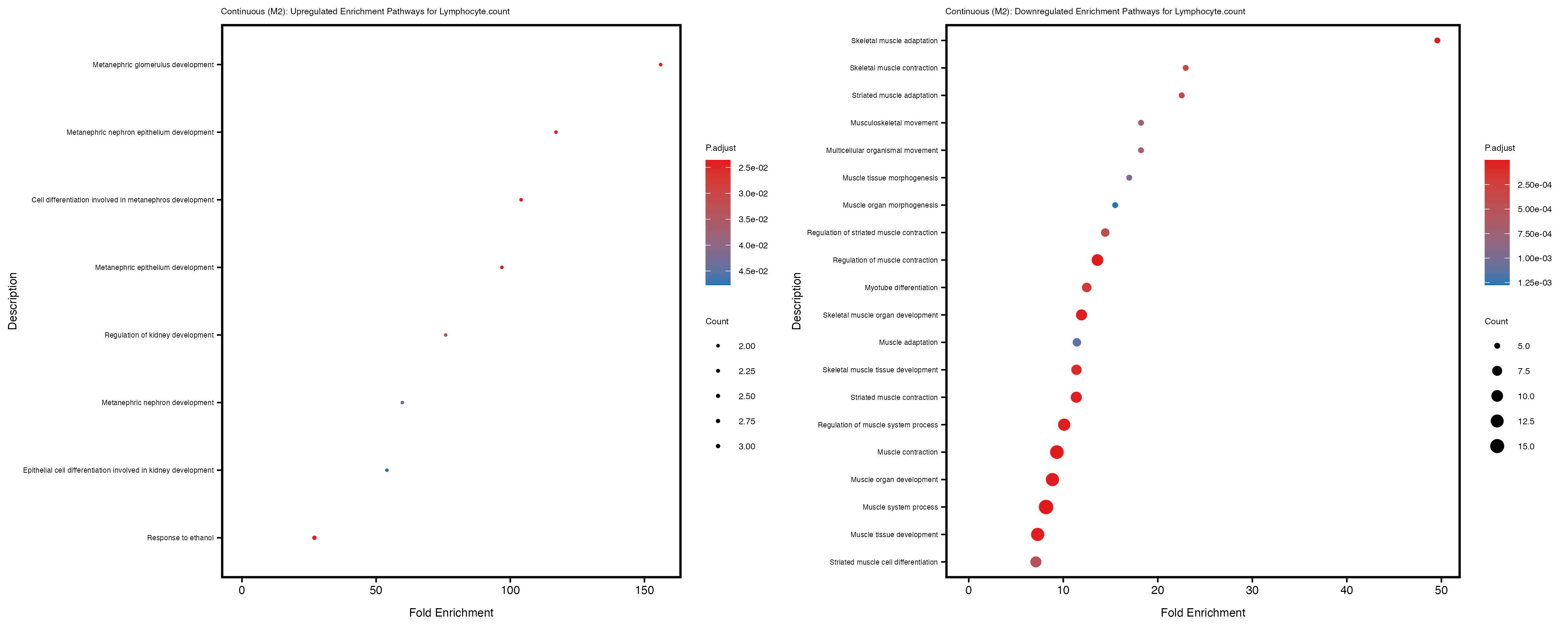
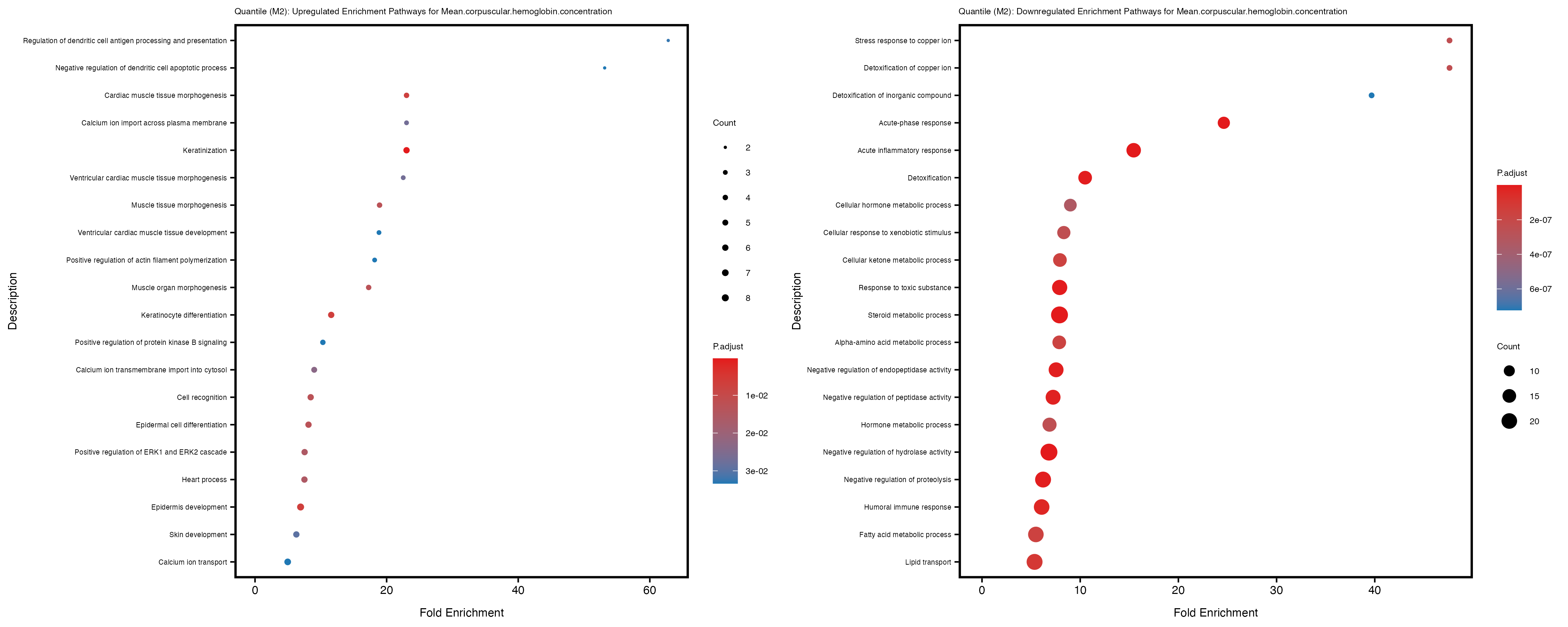
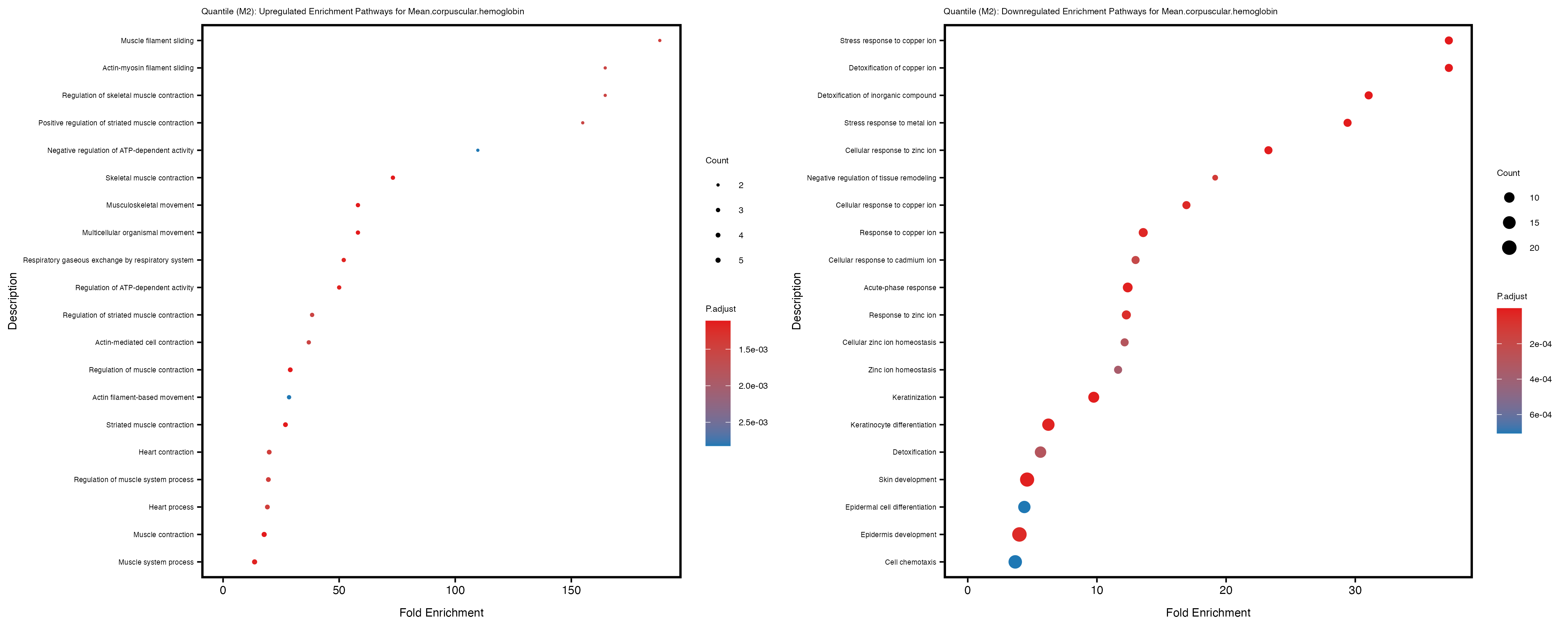
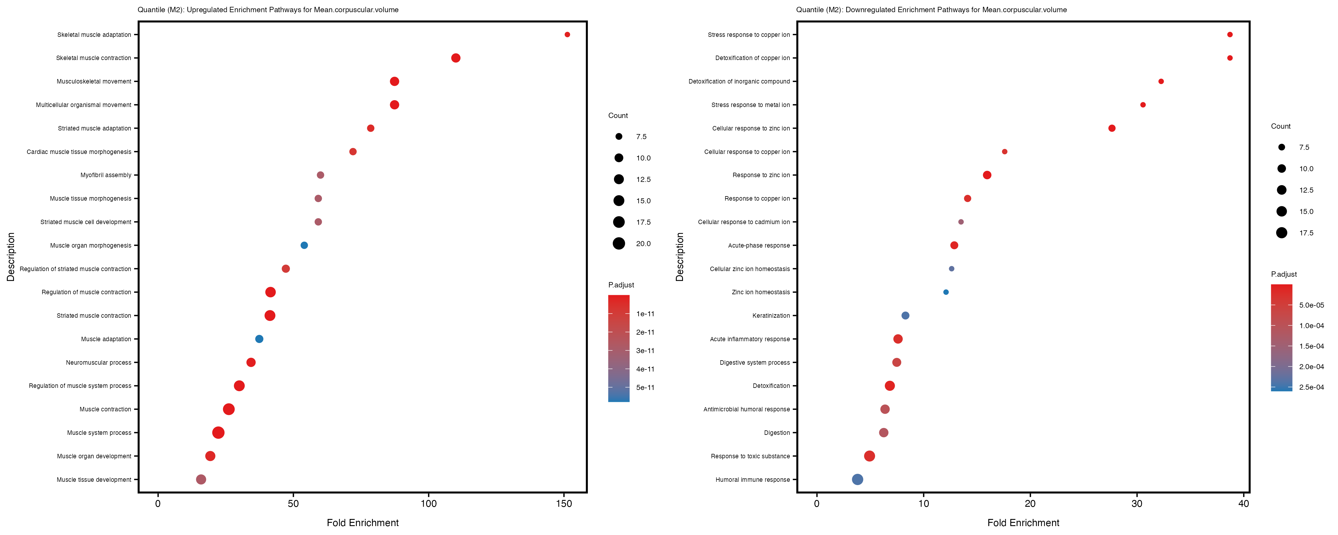
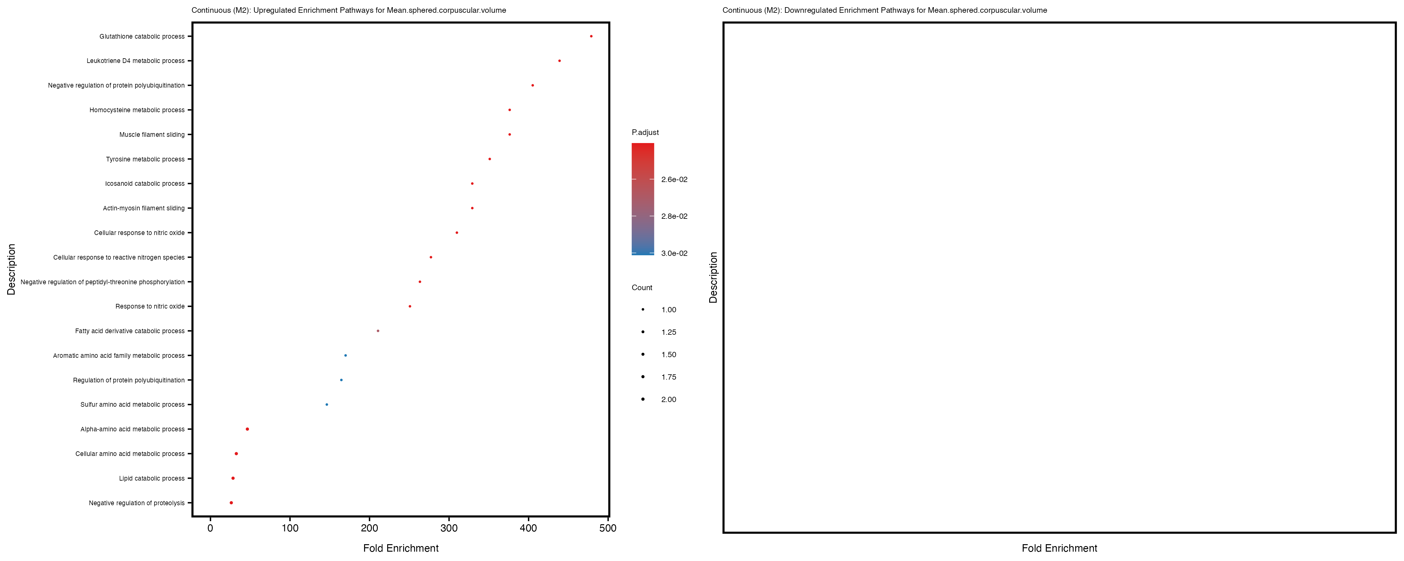
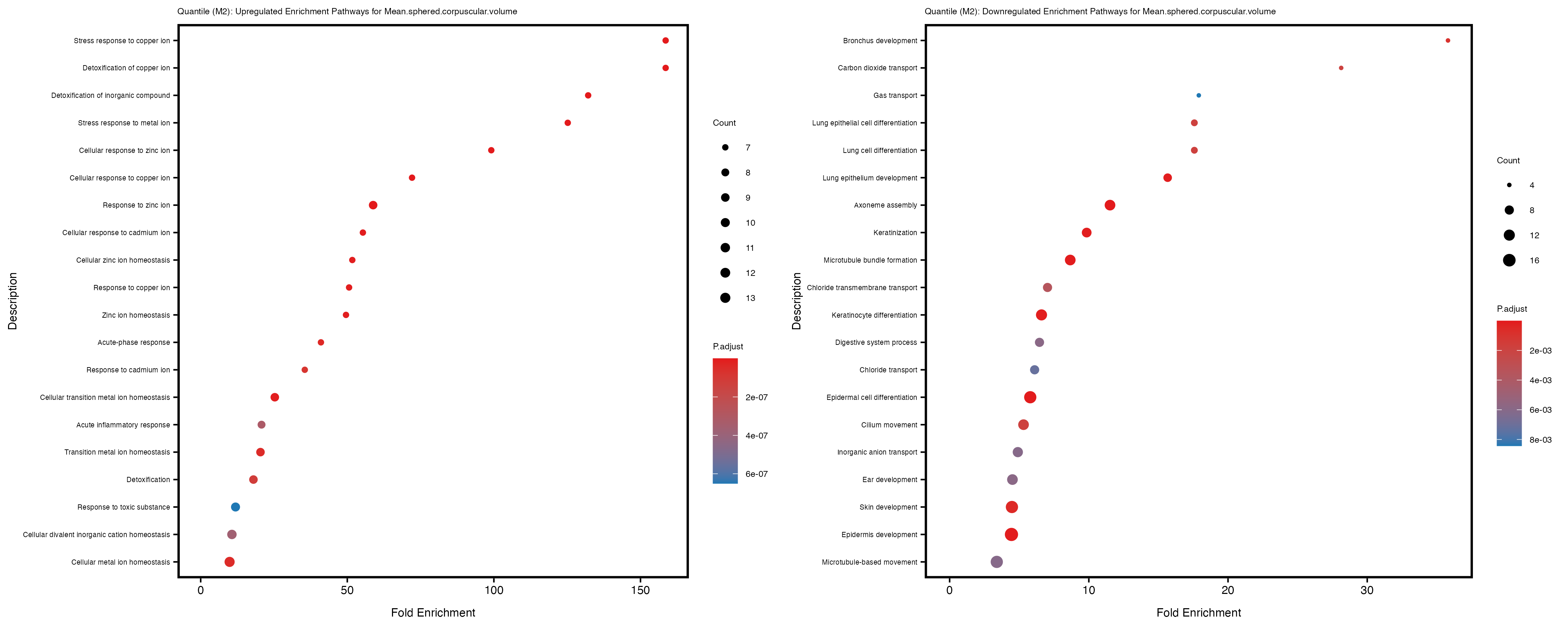
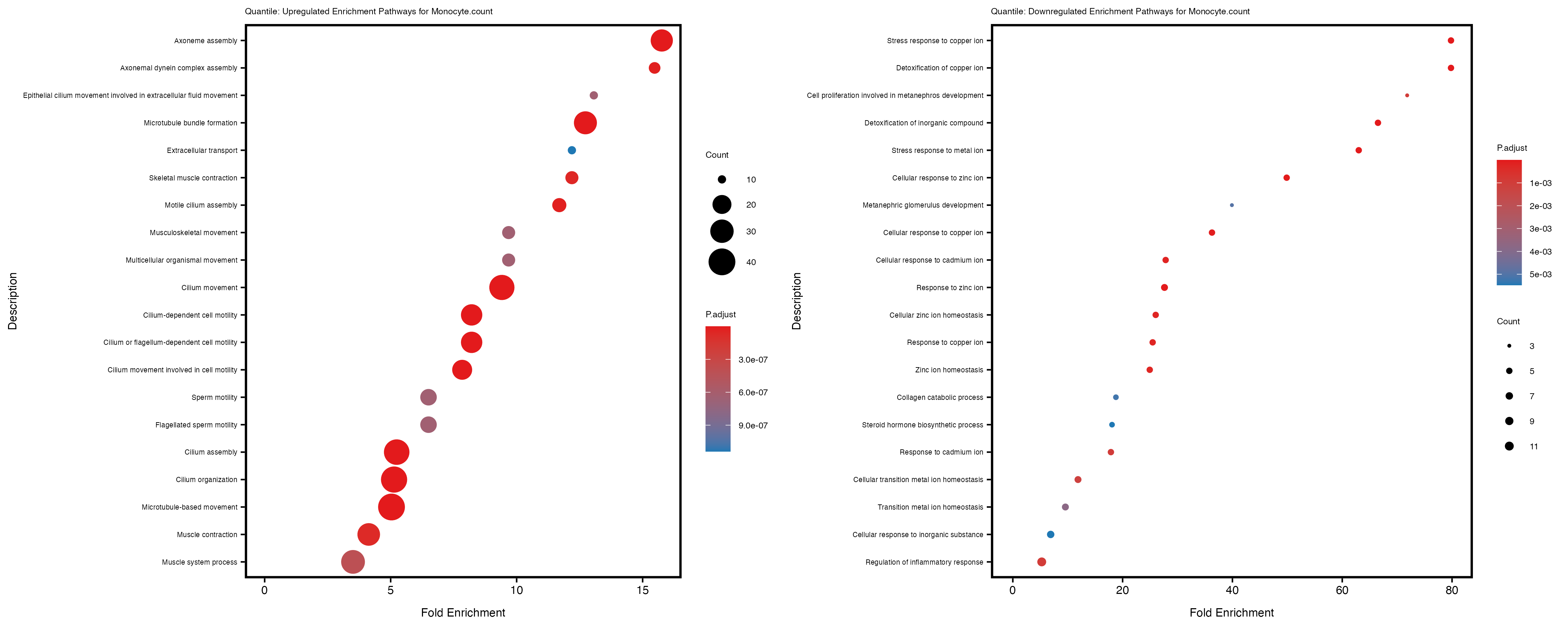
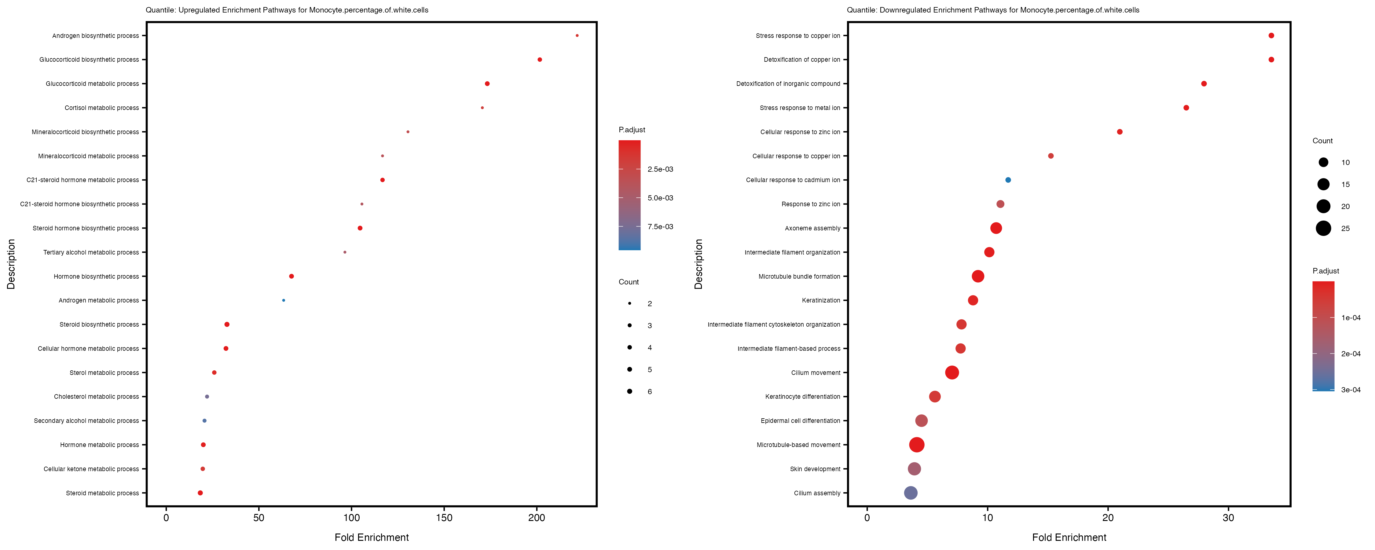
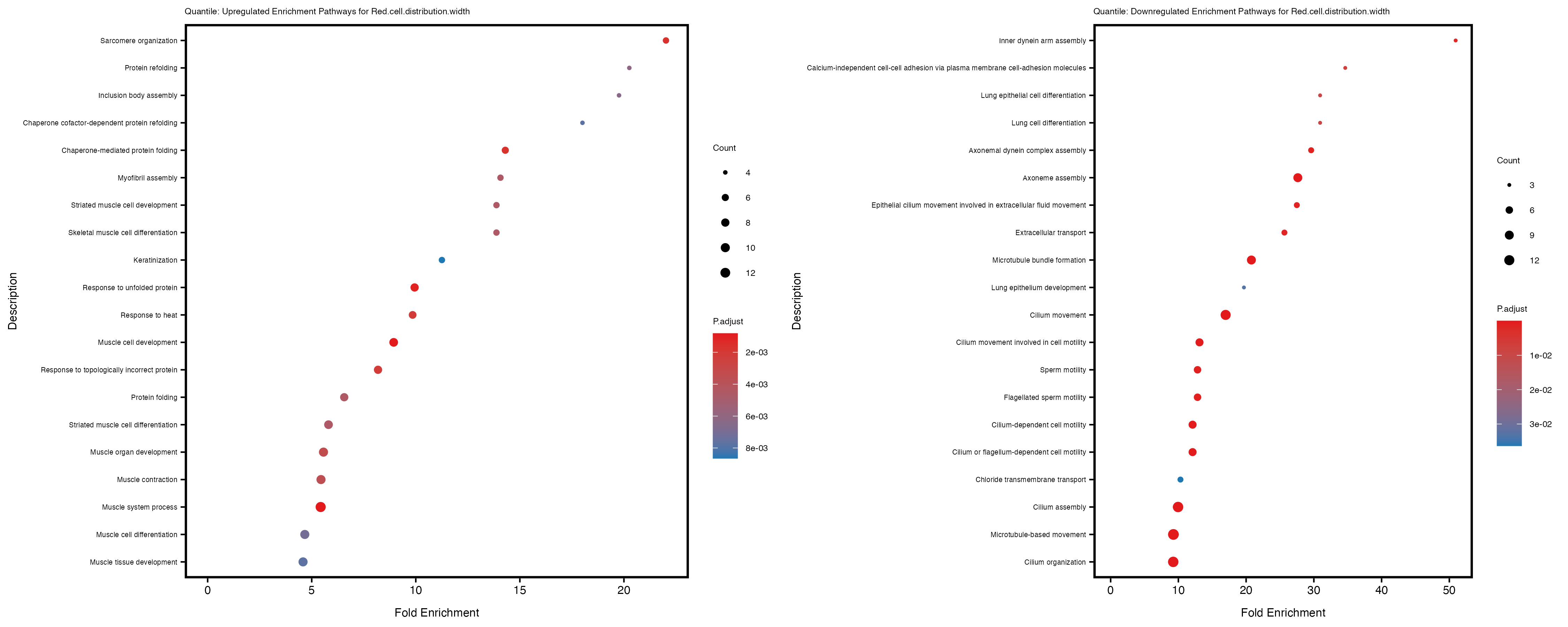
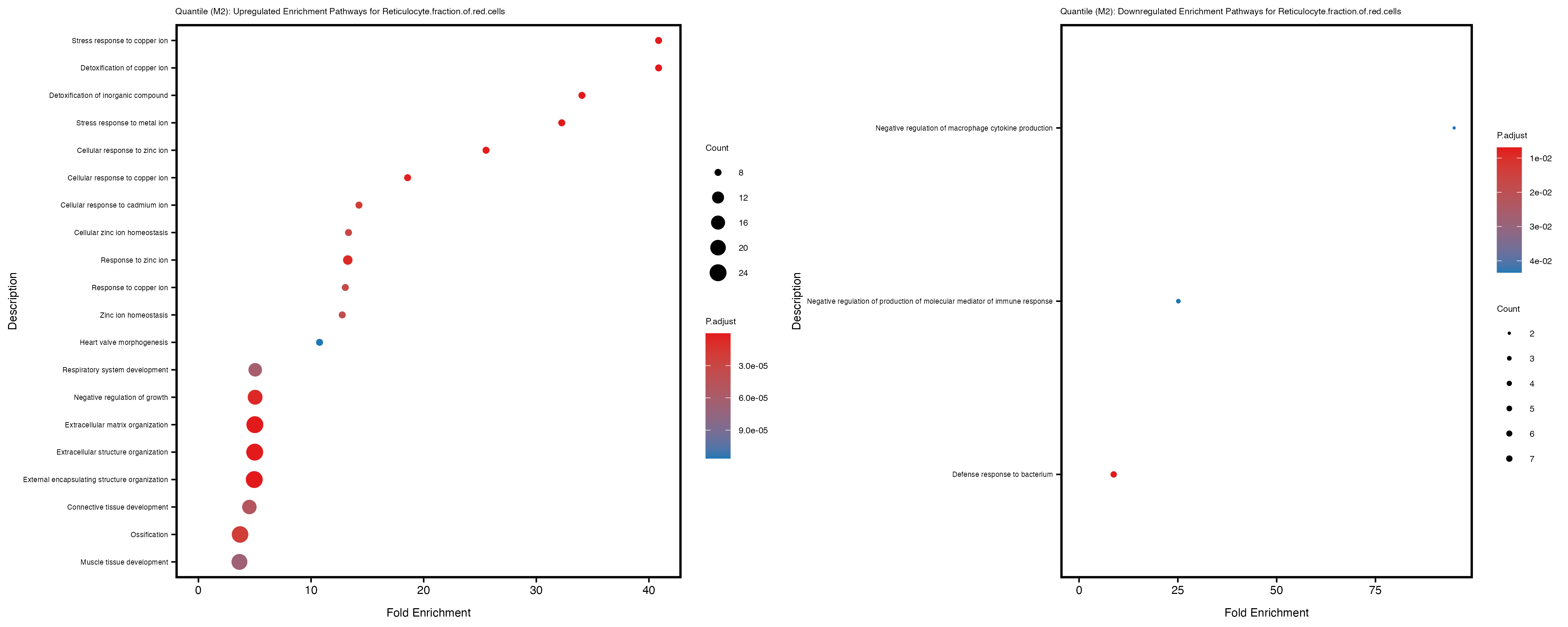
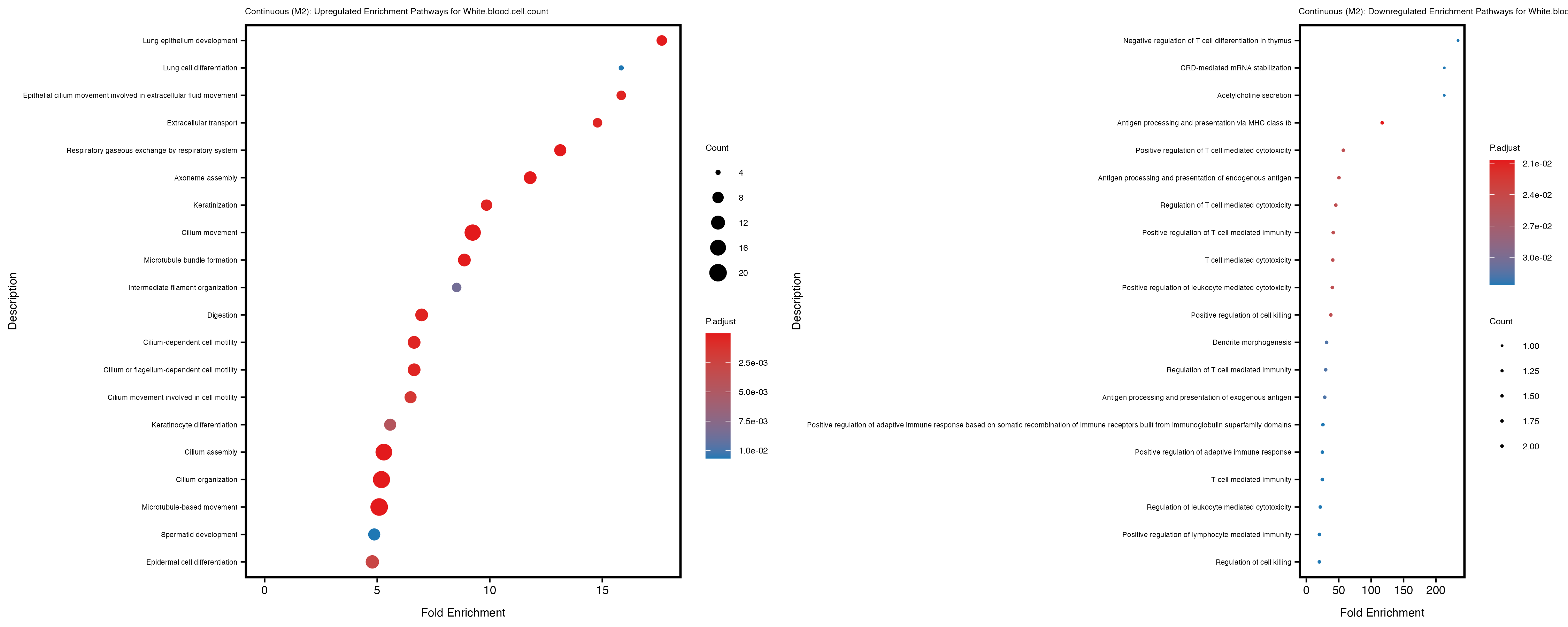
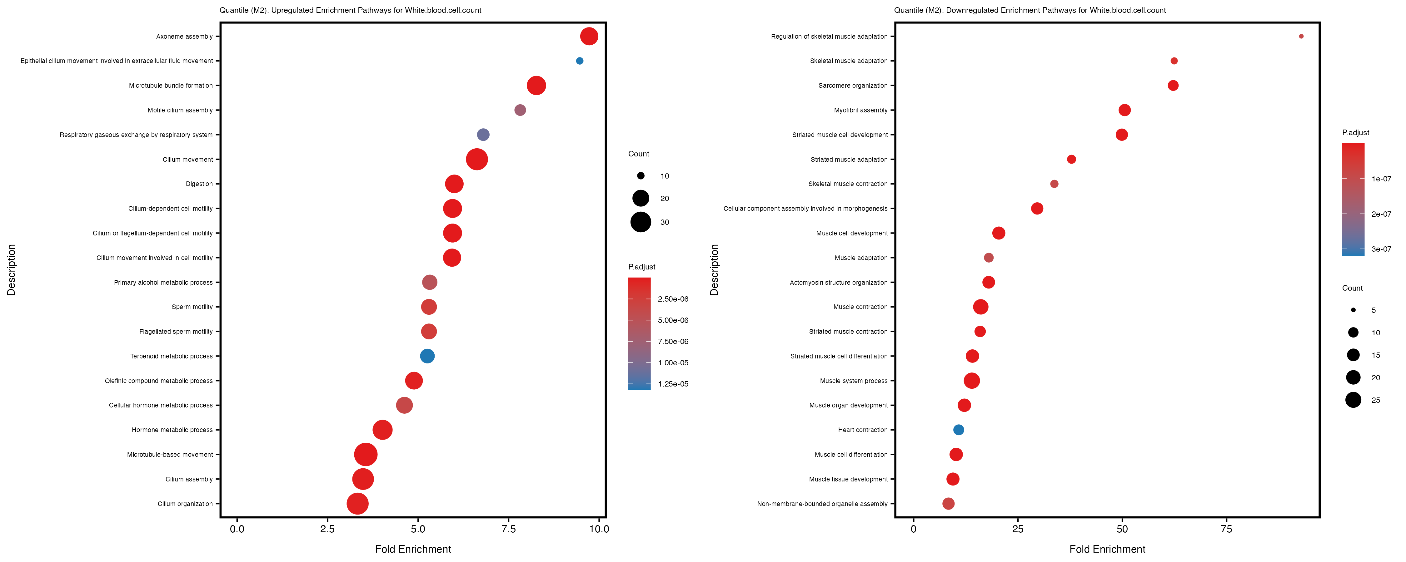
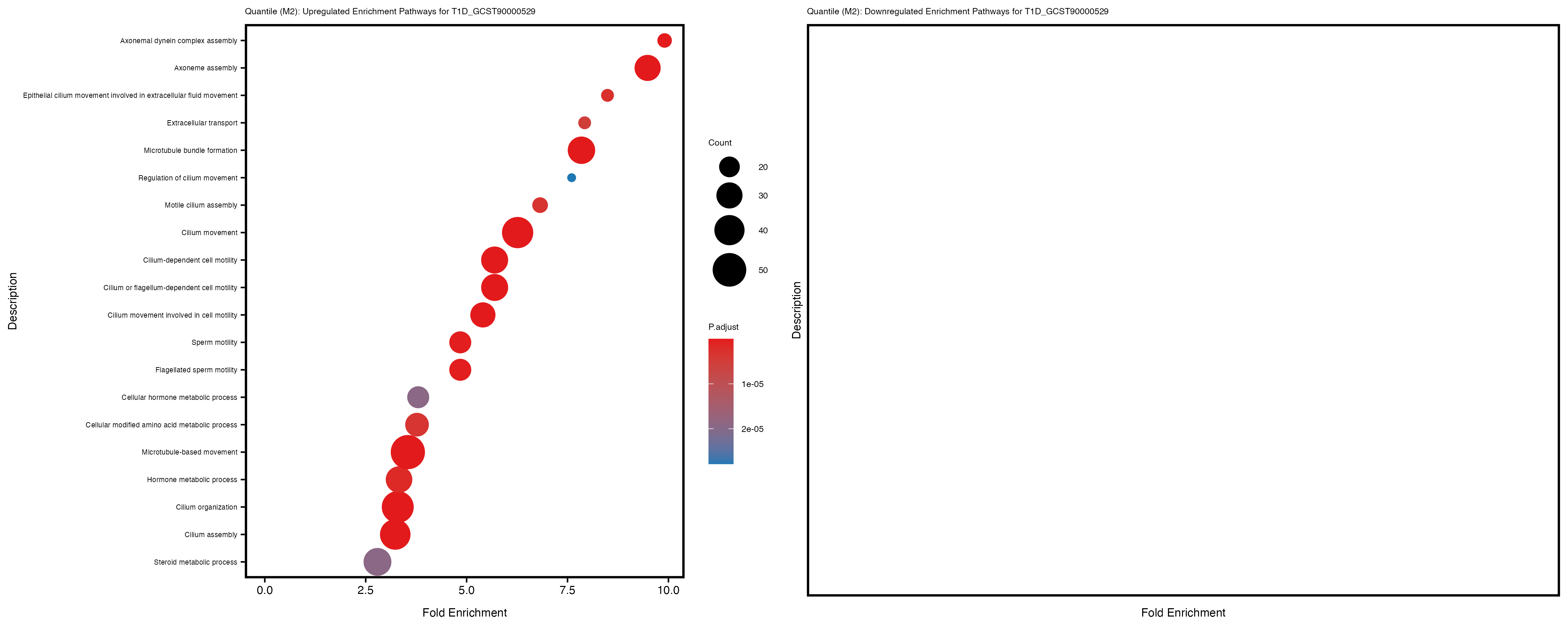
Additionally, the GO enrichment analysis provides insights into the biological pathways and processes that are potentially involved in these traits. BgRatio is the ratio of the total number of genes in a specific pathway (GO term) to the total number of genes. GeneRatio is the ratio of the number of genes enriched in specific pathway to the number of genes that were tested in the analysis. FoldEnrichment is the ratio of GeneRatio to BgRatio, showing how much more enriched a pathway is in your genes of interest compared to the total gene set. Higher FoldEnrichment values indicate that a particular GO term is overrepresented in your gene set compared to the general gene pool, suggesting it may be biologically relevant for the trait. Some traits show higher pathway enrichment in the quantile analysis, indicating that stratification by PRS may provide more biologically meaningful results.

For highly correlated traits, they tend to share similar GO enriched pathways. For example, mean corpuscular hemoglobin and mean corpucular volume are both involved in read blood cell biology, so it’s expected that their GO enrichment would point to similar biological processes, such as hemoglobin metabolism, iron homeostasis and erythropoiesis.

To account for population stratification, we adjusted the model by including the first two genotype principal components (PCs), as they explain most of the genetic variation in the data. For Eosinophil count, we observed that genes were consistently identified as top differentially expressed with and without adjustment. The only difference is that instead of SLC6A9, WFDC2 was detected as top 10 DEGs when adjusting for the first two genotype PCs. WFBC2 is a protease inhibitor with a potential role in innate immune defense (L Bingle, 2006). Although same genes are identified as top DEGs for continuous analysis, additional pathways such as response to inactivity were highlighted when adjusting for the first two genotype PCs.

Basophil count

Basophil.percentage.of.white.cells

Eosinophil.count

Eosinophil.percentage.of.white.cells

Hematocrit

Hemoglobin.concentration

High.light.scatter.reticulocyte.count

High.light.scatter.reticulocyte.percentage.of.red.cells

Immature.fraction.of.reticulocytes

Lymphocyte.count

Lymphocyte.percentage.of.white.cells

Mean.corpuscular.hemoglobin.concentration

Mean.corpuscular.hemoglobin

Mean.corpuscular.volume

Mean.platelet.volume

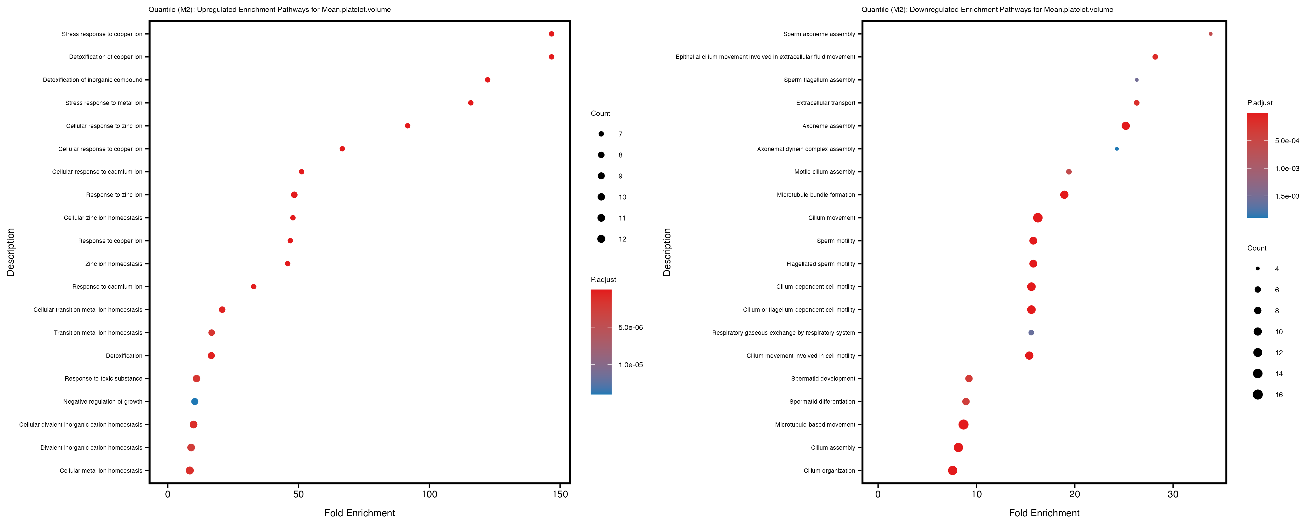
Mean.reticulocyte.volume

Mean.sphered.corpuscular.volume

Monocyte.count

Monocyte.percentage.of.white.cells

Neutrophil.count

Neutrophil.percentage.of.white.cells

Platelet.count

Platelet.crit

Platelet.distribution.width

Red.blood.cell.count

Red.cell.distribution.width

Reticulocyte.count

Reticulocyte.fraction.of.red.cells

White.blood.cell.count

Celiac_GCST90014442

Celiac_GCST90468120

IBD_GCST90013901

IBD_GCST90013951

LUPUS_GCST003156

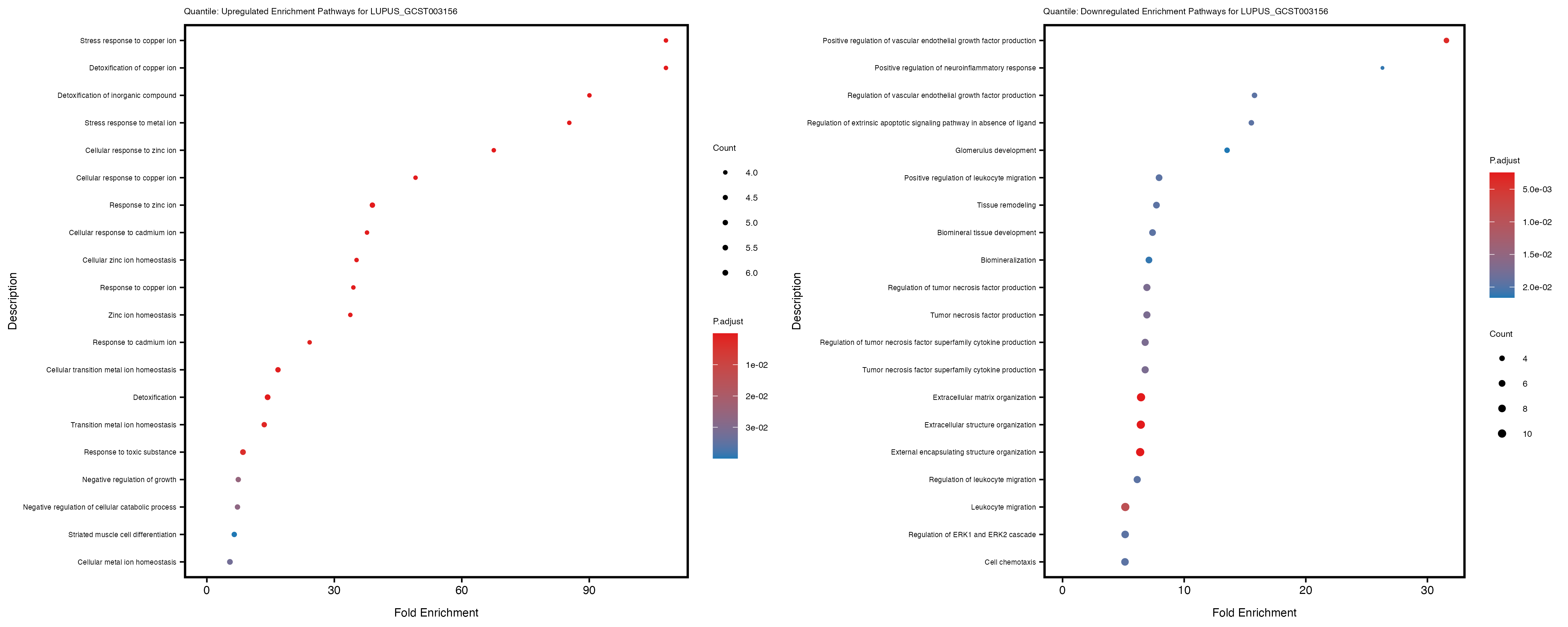
LUPUS_GCST011096

T1D_GCST90000529

T1D_GCST90014023

sessionInfo()

R version 4.2.2 (2022-10-31)
Platform: x86_64-apple-darwin17.0 (64-bit)
Running under: macOS Big Sur ... 10.16

Matrix products: default
BLAS:   /Library/Frameworks/R.framework/Versions/4.2/Resources/lib/libRblas.0.dylib
LAPACK: /Library/Frameworks/R.framework/Versions/4.2/Resources/lib/libRlapack.dylib

locale:
[1] en_US.UTF-8/en_US.UTF-8/en_US.UTF-8/C/en_US.UTF-8/en_US.UTF-8

attached base packages:
[1] stats4    stats     graphics  grDevices utils     datasets  methods  
[8] base     

other attached packages:
 [1] clusterProfiler_4.6.2       enrichplot_1.18.4          
 [3] org.Hs.eg.db_3.16.0         AnnotationDbi_1.60.2       
 [5] genekitr_1.2.8              ggrepel_0.9.6              
 [7] BiocParallel_1.32.6         DESeq2_1.38.3              
 [9] SummarizedExperiment_1.28.0 Biobase_2.58.0             
[11] MatrixGenerics_1.10.0       matrixStats_1.2.0          
[13] GenomicRanges_1.50.2        GenomeInfoDb_1.34.9        
[15] IRanges_2.32.0              S4Vectors_0.36.2           
[17] BiocGenerics_0.44.0         corrplot_0.95              
[19] ggplot2_3.5.1               dplyr_1.1.4                
[21] data.table_1.16.4           workflowr_1.7.1            

loaded via a namespace (and not attached):
  [1] shadowtext_0.1.4       fastmatch_1.1-6        plyr_1.8.9            
  [4] igraph_1.5.1           lazyeval_0.2.2         splines_4.2.2         
  [7] usethis_3.1.0          urltools_1.7.3         digest_0.6.37         
 [10] yulab.utils_0.2.0      htmltools_0.5.8.1      GOSemSim_2.24.0       
 [13] viridis_0.6.5          GO.db_3.16.0           magrittr_2.0.3        
 [16] memoise_2.0.1          remotes_2.5.0          openxlsx_4.2.5.2      
 [19] Biostrings_2.66.0      annotate_1.76.0        graphlayouts_1.0.1    
 [22] prettyunits_1.2.0      colorspace_2.1-1       blob_1.2.4            
 [25] xfun_0.50              callr_3.7.6            crayon_1.5.3          
 [28] RCurl_1.98-1.16        jsonlite_1.8.9         scatterpie_0.2.4      
 [31] ape_5.7-1              glue_1.8.0             polyclip_1.10-7       
 [34] gtable_0.3.6           zlibbioc_1.44.0        XVector_0.38.0        
 [37] DelayedArray_0.24.0    pkgbuild_1.4.6         scales_1.3.0          
 [40] DOSE_3.24.2            DBI_1.2.3              miniUI_0.1.1.1        
 [43] Rcpp_1.0.14            viridisLite_0.4.2      xtable_1.8-4          
 [46] progress_1.2.3         gridGraphics_0.5-1     tidytree_0.4.6        
 [49] bit_4.5.0.1            europepmc_0.4.3        profvis_0.4.0         
 [52] htmlwidgets_1.6.4      httr_1.4.7             fgsea_1.24.0          
 [55] RColorBrewer_1.1-3     ellipsis_0.3.2         urlchecker_1.0.1      
 [58] pkgconfig_2.0.3        XML_3.99-0.18          farver_2.1.2          
 [61] sass_0.4.9             locfit_1.5-9.8         labeling_0.4.3        
 [64] ggplotify_0.1.2        tidyselect_1.2.1       rlang_1.1.5           
 [67] reshape2_1.4.4         later_1.4.1            munsell_0.5.1         
 [70] tools_4.2.2            cachem_1.1.0           downloader_0.4        
 [73] cli_3.6.3              generics_0.1.3         RSQLite_2.3.9         
 [76] gson_0.1.0             devtools_2.4.5         evaluate_1.0.3        
 [79] stringr_1.5.1          fastmap_1.2.0          yaml_2.3.10           
 [82] ggtree_3.6.2           processx_3.8.5         knitr_1.49            
 [85] bit64_4.6.0-1          fs_1.6.5               tidygraph_1.3.0       
 [88] zip_2.3.2              purrr_1.0.2            KEGGREST_1.38.0       
 [91] ggraph_2.1.0           nlme_3.1-160           mime_0.12             
 [94] whisker_0.4.1          aplot_0.2.4            ggvenn_0.1.10         
 [97] xml2_1.3.6             compiler_4.2.2         rstudioapi_0.17.1     
[100] png_0.1-8              treeio_1.22.0          tibble_3.2.1          
[103] tweenr_2.0.3           geneplotter_1.76.0     bslib_0.9.0           
[106] stringi_1.8.4          ps_1.8.1               lattice_0.22-6        
[109] Matrix_1.6-4           vctrs_0.6.5            pillar_1.10.1         
[112] lifecycle_1.0.4        triebeard_0.4.1        jquerylib_0.1.4       
[115] cowplot_1.1.3          bitops_1.0-9           httpuv_1.6.15         
[118] patchwork_1.3.0        qvalue_2.30.0          R6_2.5.1              
[121] promises_1.3.2         gridExtra_2.3          sessioninfo_1.2.2     
[124] codetools_0.2-20       pkgload_1.4.0          MASS_7.3-58.1         
[127] rprojroot_2.0.4        withr_3.0.2            GenomeInfoDbData_1.2.9
[130] parallel_4.2.2         hms_1.1.3              grid_4.2.2            
[133] ggfun_0.1.8            tidyr_1.3.1            HDO.db_0.99.1         
[136] rmarkdown_2.29         git2r_0.33.0           getPass_0.2-4         
[139] ggforce_0.4.1          shiny_1.10.0           geneset_0.2.7

Differential expression

Correlation between PRS & expression PCs (whole blood)

Perform DESeq2 differential expression analysis for each trait

Model 1: expression ~ PRS + sex + expression PCs

Model 2: expression ~ PRS + sex + expression PCs + 2 genotype PCs

GO enrichment Analysis

Result

Summary table

Basophil count

Basophil.percentage.of.white.cells

Eosinophil.count

Eosinophil.percentage.of.white.cells

Hematocrit

Hemoglobin.concentration

High.light.scatter.reticulocyte.count

High.light.scatter.reticulocyte.percentage.of.red.cells

Immature.fraction.of.reticulocytes

Lymphocyte.count

Lymphocyte.percentage.of.white.cells

Mean.corpuscular.hemoglobin.concentration

Mean.corpuscular.hemoglobin

Mean.corpuscular.volume

Mean.platelet.volume

Mean.reticulocyte.volume

Mean.sphered.corpuscular.volume

Monocyte.count

Monocyte.percentage.of.white.cells

Neutrophil.count

Neutrophil.percentage.of.white.cells

Platelet.count

Platelet.crit

Platelet.distribution.width

Red.blood.cell.count

Red.cell.distribution.width

Reticulocyte.count

Reticulocyte.fraction.of.red.cells

White.blood.cell.count

Celiac_GCST90014442

Celiac_GCST90468120

IBD_GCST90013901

IBD_GCST90013951

LUPUS_GCST003156

LUPUS_GCST011096

T1D_GCST90000529

T1D_GCST90014023