Normalization gene counts
Last updated: 2025-04-24
Checks: 7 0
Knit directory: prs/
This reproducible R Markdown analysis was created with workflowr (version 1.7.1). The Checks tab describes the reproducibility checks that were applied when the results were created. The Past versions tab lists the development history.
Great! Since the R Markdown file has been committed to the Git repository, you know the exact version of the code that produced these results.
Great job! The global environment was empty. Objects defined in the global environment can affect the analysis in your R Markdown file in unknown ways. For reproduciblity it’s best to always run the code in an empty environment.
The command set.seed(20250417) was run prior to running
the code in the R Markdown file. Setting a seed ensures that any results
that rely on randomness, e.g. subsampling or permutations, are
reproducible.
Great job! Recording the operating system, R version, and package versions is critical for reproducibility.
Nice! There were no cached chunks for this analysis, so you can be confident that you successfully produced the results during this run.
Great job! Using relative paths to the files within your workflowr project makes it easier to run your code on other machines.
Great! You are using Git for version control. Tracking code development and connecting the code version to the results is critical for reproducibility.
The results in this page were generated with repository version 077b30f. See the Past versions tab to see a history of the changes made to the R Markdown and HTML files.
Note that you need to be careful to ensure that all relevant files for
the analysis have been committed to Git prior to generating the results
(you can use wflow_publish or
wflow_git_commit). workflowr only checks the R Markdown
file, but you know if there are other scripts or data files that it
depends on. Below is the status of the Git repository when the results
were generated:
Ignored files:
    Ignored:    .DS_Store
    Ignored:    .Rhistory
    Ignored:    .Rproj.user/
    Ignored:    analysis/.DS_Store
    Ignored:    data/.DS_Store

Untracked files:
    Untracked:  analysis/dds.rda
    Untracked:  analysis/differential_expression.Rmd
    Untracked:  analysis/metadata.txt
    Untracked:  analysis/normalized_counts.rda
    Untracked:  analysis/vst norm counts.rda
    Untracked:  data/GTEx_v8.bk
    Untracked:  data/GTEx_v8.rds
    Untracked:  data/Whole_Blood.v8.covariates.txt
    Untracked:  data/blood_cell/
    Untracked:  data/gene_reads_2017-06-05_v8_whole_blood.gct
    Untracked:  data/gene_tpm_2017-06-05_v8_whole_blood.gct.gz
    Untracked:  data/immune/

Unstaged changes:
    Deleted:    analysis/normalized_counts.txt
    Modified:   prs.Rproj
Note that any generated files, e.g. HTML, png, CSS, etc., are not included in this status report because it is ok for generated content to have uncommitted changes.
These are the previous versions of the repository in which changes were
made to the R Markdown
(analysis/expression_normalization.Rmd) and HTML
(docs/expression_normalization.html) files. If you’ve
configured a remote Git repository (see ?wflow_git_remote),
click on the hyperlinks in the table below to view the files as they
were in that past version.
| File | Version | Author | Date | Message |
|---|---|---|---|---|
| Rmd | 077b30f | ElisaChen | 2025-04-24 | wflow_publish(c("analysis/index.Rmd", "analysis/about.Rmd", "analysis/license.Rmd", |
| Rmd | 7338250 | ElisaChen | 2025-04-17 | first commit |
Raw count
# Load the gene expression data
gene_expr_file <- "data/gene_reads_2017-06-05_v8_whole_blood.gct"
raw_count_df <- fread(gene_expr_file, header = TRUE)

gene_name <- raw_count_df$Description
raw_count_df <- raw_count_df[, -c(1:3)]

# modify GTEx sample names matching names used in PRS data
colnames(raw_count_df) <- sub("^(GTEX-[^-.]+).*", "\\1", colnames(raw_count_df))

# load metadata
metadata_file <- "analysis/metadata.txt"
metadata <- read.csv(metadata_file, header = T, sep = "\t", stringsAsFactors = T)
metadata$sex <- as.factor(metadata$sex)
matching_samples <- intersect(rownames(metadata), colnames(raw_count_df))
final_count <- raw_count_df[ , ..matching_samples]
dim(final_count)
[1] 56200 670Create DESeq2 object
# Create the DESeq2 object (DESeqDataSet) from the raw count matrix and PRS
group_columns <- grep("^group_", colnames(metadata), value = TRUE)
dds <- DESeqDataSetFromMatrix(countData = as.matrix(final_count),
                              colData = metadata,
                              design = as.formula(paste("~ PC1 + PC2 + PC3 + PC4 + PC5 + sex +",
                                                        paste(group_columns, collapse = " + "))))
rownames(dds) <- gene_name

# prefilter: keep only rows that have a count of at least 10 for a minimal number of samples
keep_genes <- rowSums(counts(dds) >= 10) >= 100
dds <- dds[keep_genes, ]
#save(dds, file = "analysis/dds.rda")
Estimate size factors for normalization
dds <- estimateSizeFactors(dds)
outliers <- which(sizeFactors(dds) > 4)
plot(sizeFactors(dds), colSums(counts(dds)), ylab = "library sizes",
     xlab = "size factors", cex = .5)
text(sizeFactors(dds)[outliers], colSums(counts(dds))[outliers],
     labels = colnames(dds)[outliers], pos = 2, cex = .5, col = "red")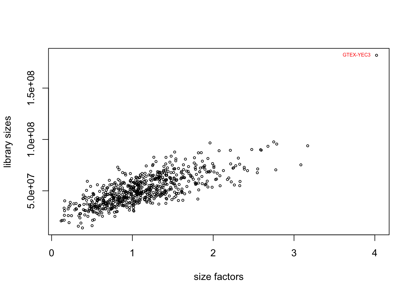
The plot suggests a positive correlation between the library sizes and size factors, indicating that samples with higher total counts tend to have higher size factors. The sample GTEX-YEC3 is an outlier. GTEX-YEC3 may have significantly different sequencing characteristics, leading to a higher library size and size factor compared to the other samples.
To address this issue of the outlier and sequencing depth, we apply two normalization methods:
1. DESeq2 normalization by median of ratios
The size factor is calculated as follows:
For each gene, the geometric mean of counts across all samples is computed (this serves as the pseudo baseline expression).
For each gene, the ratio of its count in a specific sample to the pseudo-baseline expression is calculated (e.g., Sample A/pseudo baseline, Sample B/pseudo baseline).
For each sample, the median of these ratios is computed, which results in the size factor for that sample.
Thus, DESeq2 normalizes for both sequencing depth and RNA composition differences, and this process is independent of the design matrix, meaning it is unaffected by the specific traits (whether blood or immune traits) used in the analysis.
# obtain normalized counts
normalized_counts <- counts(dds, normalized=TRUE)
#save(normalized_counts, file = "analysis/normalized_counts.rda")
2. TPM Quantile normalization
# load TPM counts data
tpm_file <- "data/gene_tpm_2017-06-05_v8_whole_blood.gct.gz"
tpm_count_df <- fread(tpm_file, header = TRUE, stringsAsFactors = FALSE)
colnames(tpm_count_df) <- sub("^(GTEX-[^-.]+).*", "\\1", colnames(tpm_count_df))

# subset samples & remove no read genes
tpm_subset_df <- tpm_count_df[, matching_samples, with = FALSE]
# Keep rows with at least 10 counts in at least 100 samples
tpm_subset_df <- tpm_subset_df[rowSums(tpm_subset_df[, -1, with = FALSE] >= 10) >= 100, ]

# convert into matrix
tpm_count <- as.matrix(tpm_subset_df)

# perform quantile normalization
qn_counts <- preprocessCore::normalize.quantiles(tpm_count)
colnames(qn_counts) <- matching_samples
Compare raw counts, DESeq2 normalized count & quantile normalized count
boxplot(log2(counts(dds) + 1)[, c(1:10, outliers)],
        main = "Raw read counts", ylab = "log2(read counts)", cex = .6,
col = c(rep("lightblue", 10), "red"), las = 2) 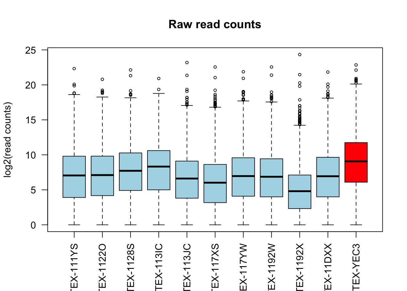
boxplot(log2(counts(dds, normalize = TRUE) + 1)[, c(1:10, outliers)],
        main = "DESeq2 normalized read counts", ylab = "log2(read counts)",
        cex = .6, col = c(rep("lightblue", 10), "red"), las = 2)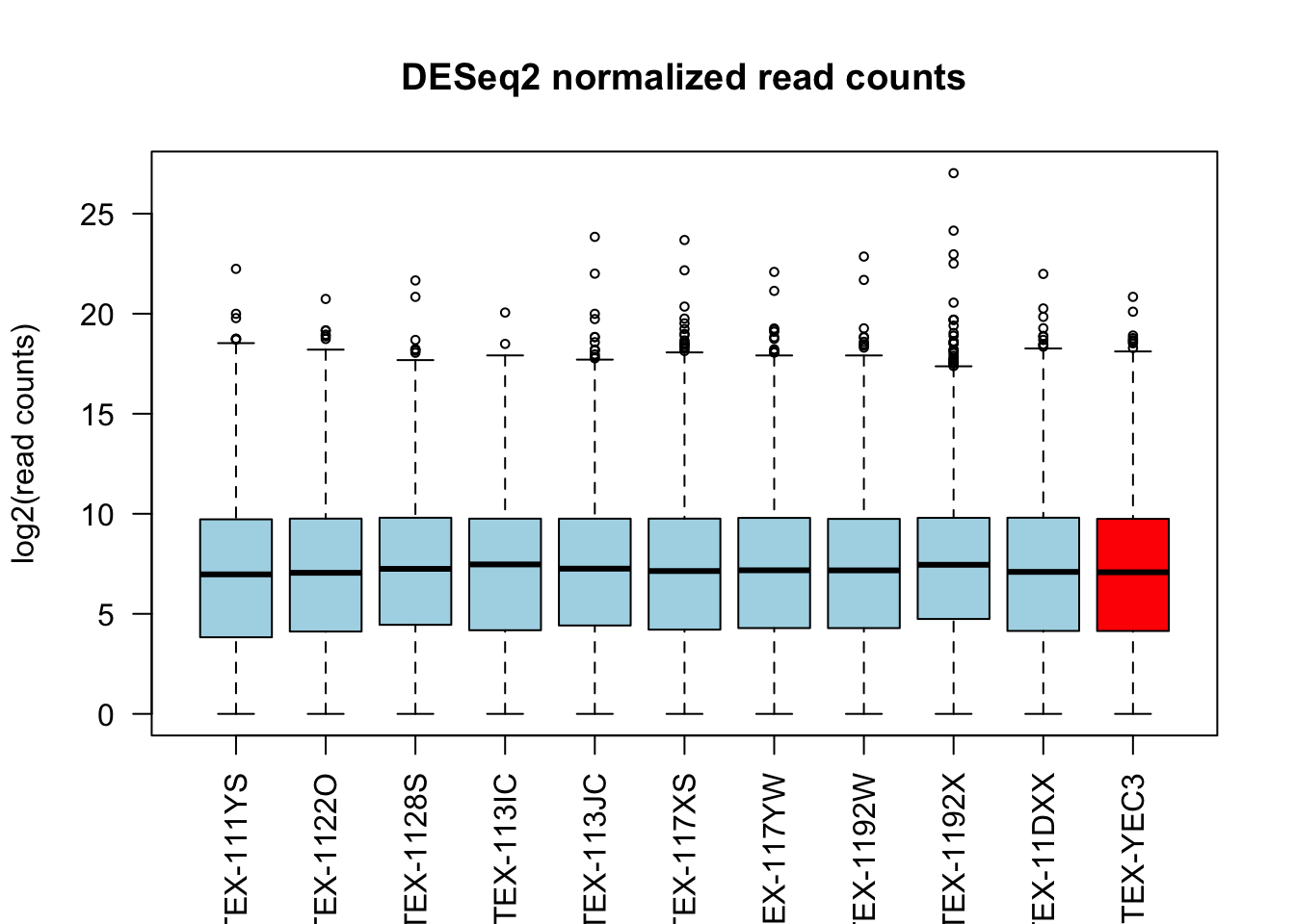
boxplot(log2(qn_counts + 1)[, c(1:10, outliers)],
        main = "Quantile normalized read counts", ylab = "log2(read counts)",
cex = .6, col = c(rep("lightblue", 10), "red"), las = 2) 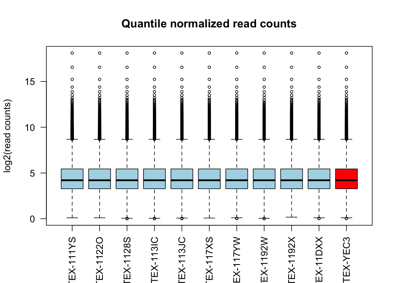
Both normalization methods successfully adjust for the differences in sequencing depth across samples.
Correlation between outlier with other samples after normalization
1. DESeq2 normalized counts
assay(dds, "log.counts") <- log2(counts(dds, normalized = FALSE) + 1)
assay(dds, "log.norm.counts") <- log2(counts(dds, normalized=TRUE) + 1)

par(mfrow=c(1,2))
dds[, c("GTEX-YEC3", "GTEX-111YS")] %>%
  assay(., "log.norm.counts") %>%
  plot(., cex=.1, main = "GTEX-YEC3 vs GTEX-111YS")

dds[, c("GTEX-YEC3", "GTEX-1122O")] %>%
  assay(., "log.norm.counts") %>%
  plot(., cex=.1, main = "GTEX-YEC3 vs GTEX-1122O")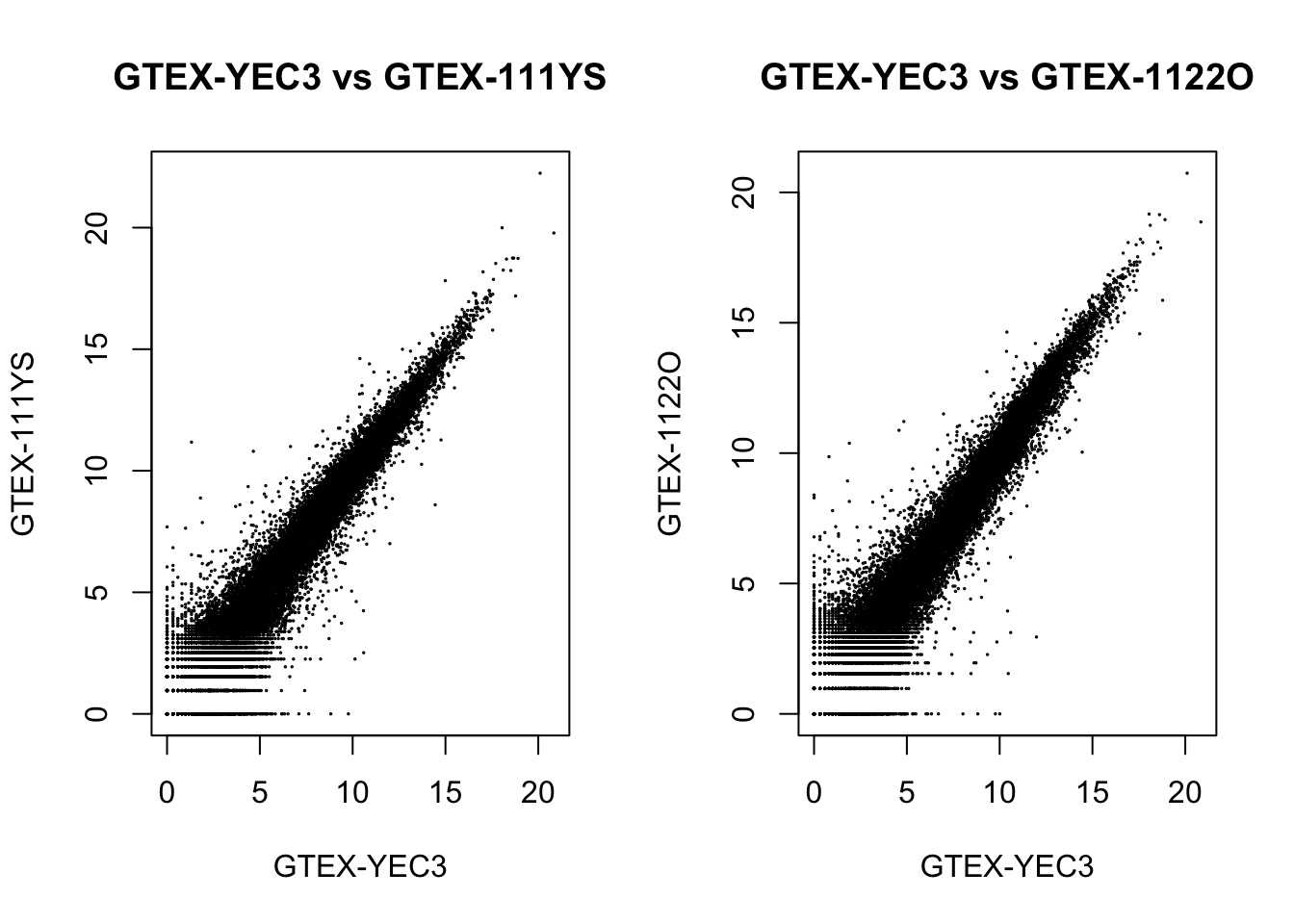
dds[, c("GTEX-YEC3", "GTEX-YEC4")] %>%
  assay(., "log.norm.counts") %>%
  plot(., cex=.1, main = "GTEX-YEC3 vs GTEX-YEC4")

dds[, c("GTEX-YEC3", "GTEX-YBZK")] %>%
  assay(., "log.norm.counts") %>%
  plot(., cex=.1, main = "GTEX-YEC3 vs GTEX-YBZK")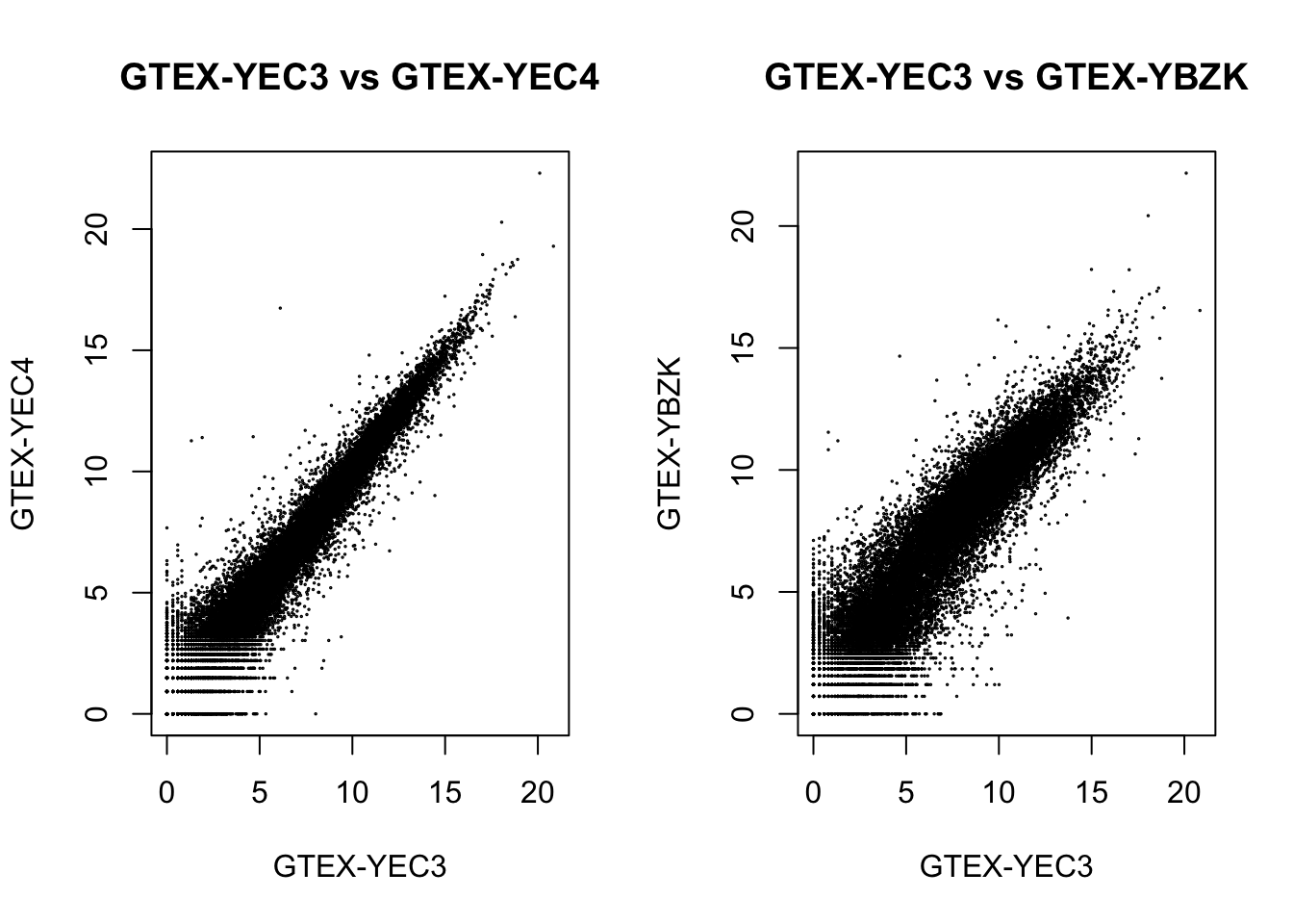
2. Quantile Normalization
log2_qn_counts <- log2(qn_counts + 1)

par(mfrow=c(1,2))
plot(log2_qn_counts[, "GTEX-YEC3"], log2_qn_counts[, "GTEX-111YS"], cex=.1,
      main = "GTEX-YEC3 vs GTEX-111YS", xlab = "GTEX-YEC3", ylab = "GTEX-111YS")

plot(log2_qn_counts[, "GTEX-YEC3"], log2_qn_counts[, "GTEX-1122O"], cex=.1,
      main = "GTEX-YEC3 vs GTEX-1122O", xlab = "GTEX-YEC3", ylab = "GTEX-1122O")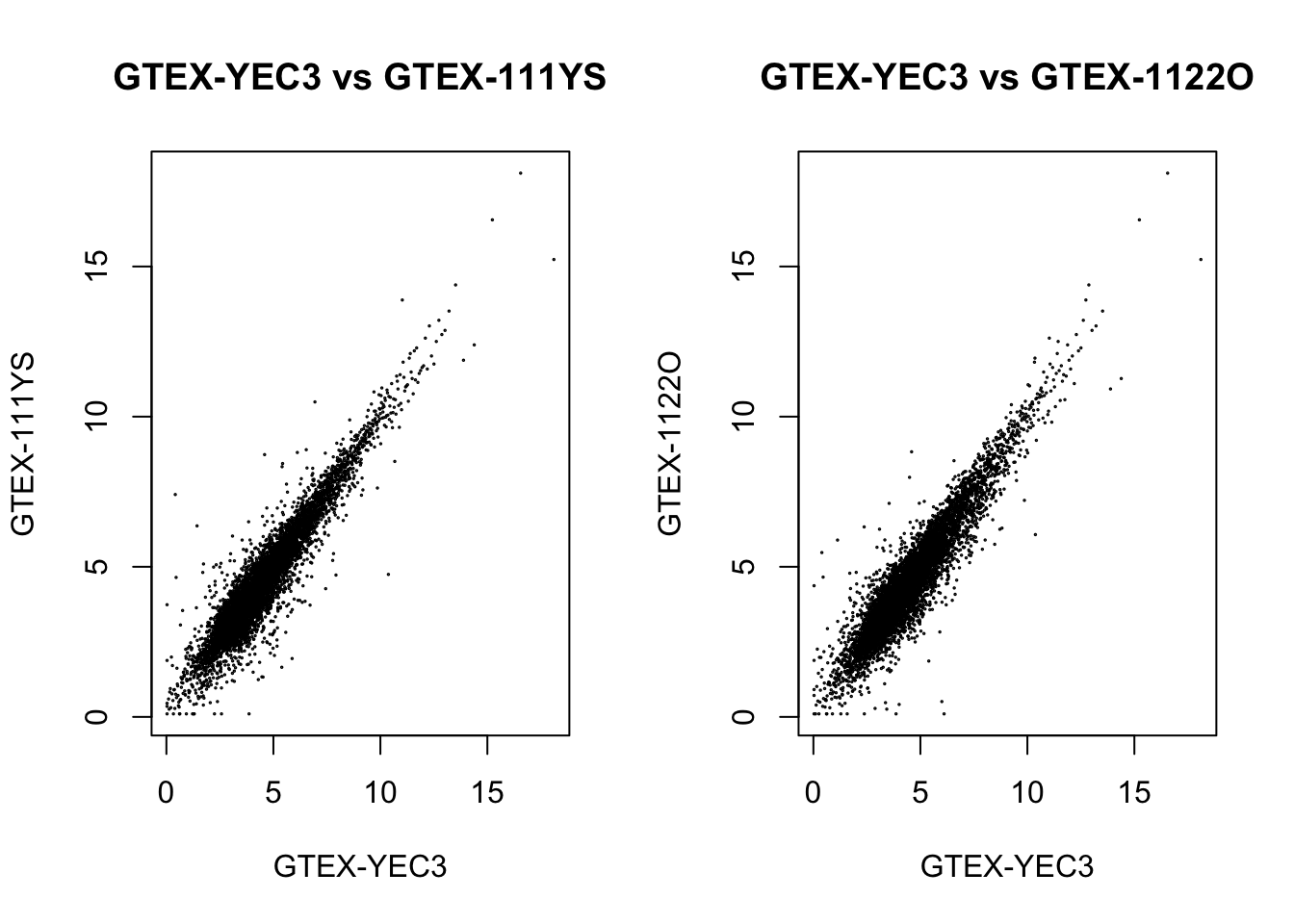
plot(log2_qn_counts[, "GTEX-YEC3"], log2_qn_counts[, "GTEX-YEC4"], cex=.1,
      main = "GTEX-YEC3 vs GTEX-YEC4", xlab = "GTEX-YEC3", ylab = "GTEX-YEC4")

plot(log2_qn_counts[, "GTEX-YEC3"], log2_qn_counts[, "GTEX-YBZK"], cex=.1,
      main = "GTEX-YEC3 vs GTEX-YBZK", xlab = "GTEX-YEC3", ylab = "GTEX-YBZK")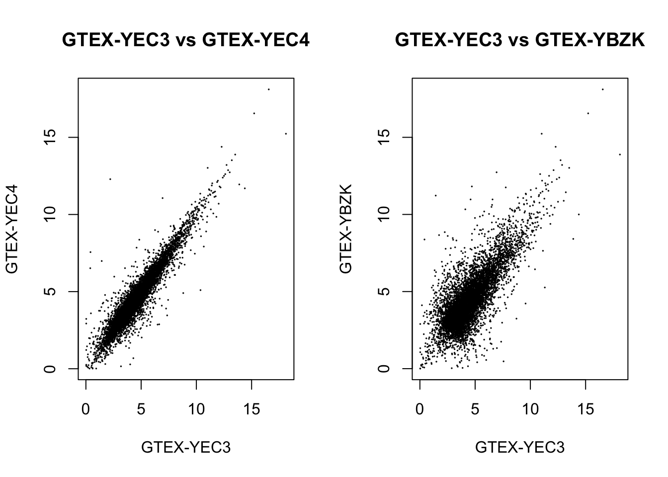
We could see a positive correlation between the outlier with other samples after applying either normalization methods, so the outlier shouldn’t be an effect.
From the DESeq2 normalization plot, we see a fanning out pattern for points before \(2^5 = 32\), suggesting that read counts correlate less well when they are low. The observation also implies that the standard deviation of the expression levels may depend on the mean: the lower the mean read counts per gene, the higher the standard deviation.
Reduce the dependence of the variance on the mean
# mean & sd relationship
log.norm.counts <- log2(counts(dds, normalized=TRUE) + 1)

msd_plot <- vsn::meanSdPlot(log.norm.counts,
                            ranks=FALSE,
                            plot = FALSE)
msd_plot$gg +
  ggtitle("Sequencing depth normalized log2(read counts)") +
  ylab("standard deviation")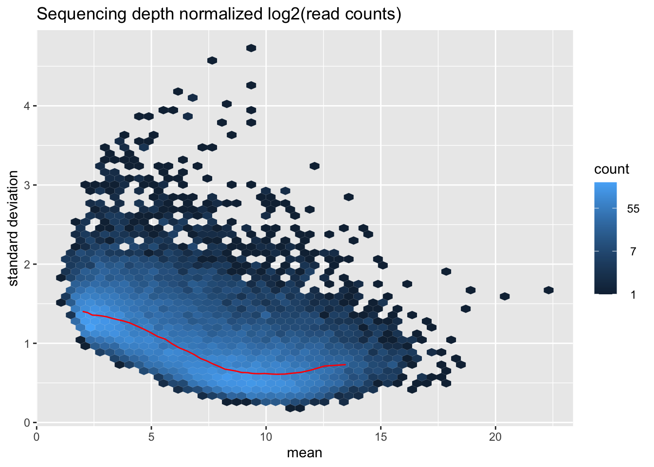
Given the large sample size of 670, we use varianceStabilizingTransformation (vst) to log-transformed counts for genes with very counts.
# reduce variance dependent on mean
dds.vsd <- vst(dds, blind=FALSE)
save(dds.vsd, file = "analysis/vst norm counts.rda")
load("analysis/vst norm counts.rda")
vsd.norm.counts <- assay(dds.vsd)
par(mfrow=c(1,2))
plot(log.norm.counts[,1:2], cex=.1, main = "log2-transformed")
plot(vsd.norm.counts[,1], vsd.norm.counts[,2], cex=.1, main = "Variance Stabilizing Transformed",
xlab = colnames(vsd.norm.counts[,1]),
ylab = colnames(vsd.norm.counts[,1]))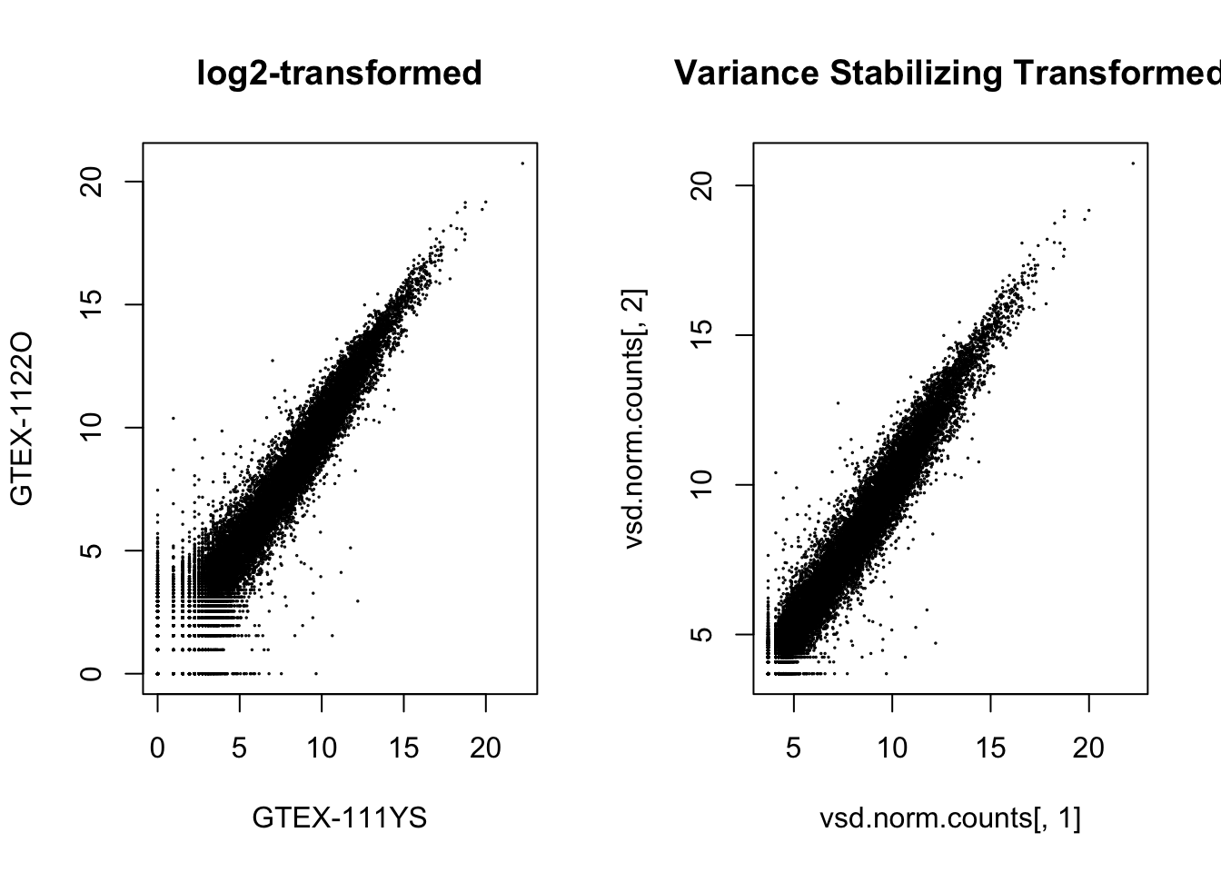
msd_plot <- vsn::meanSdPlot(vsd.norm.counts, ranks=FALSE, plot = FALSE)
msd_plot$gg + ggtitle("vst transformation") + coord_cartesian(ylim = c(0,4))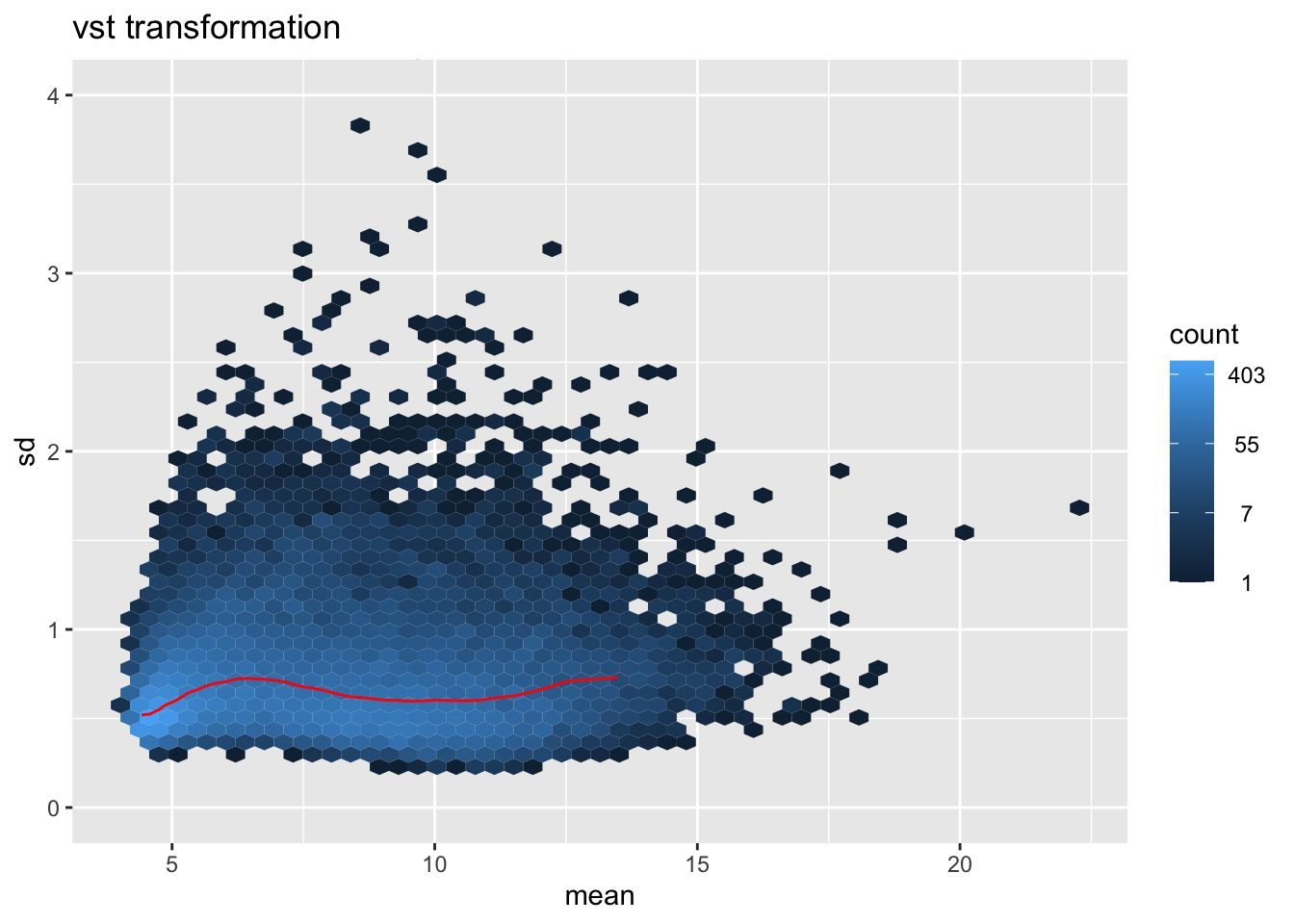
sessionInfo()R version 4.2.2 (2022-10-31)
Platform: x86_64-apple-darwin17.0 (64-bit)
Running under: macOS Big Sur ... 10.16
Matrix products: default
BLAS: /Library/Frameworks/R.framework/Versions/4.2/Resources/lib/libRblas.0.dylib
LAPACK: /Library/Frameworks/R.framework/Versions/4.2/Resources/lib/libRlapack.dylib
locale:
[1] en_US.UTF-8/en_US.UTF-8/en_US.UTF-8/C/en_US.UTF-8/en_US.UTF-8
attached base packages:
[1] stats4 stats graphics grDevices utils datasets methods
[8] base
other attached packages:
[1] tidyr_1.3.1 ggplot2_3.5.1
[3] preprocessCore_1.60.2 DESeq2_1.38.3
[5] SummarizedExperiment_1.28.0 Biobase_2.58.0
[7] MatrixGenerics_1.10.0 matrixStats_1.2.0
[9] GenomicRanges_1.50.2 GenomeInfoDb_1.34.9
[11] IRanges_2.32.0 S4Vectors_0.36.2
[13] BiocGenerics_0.44.0 dplyr_1.1.4
[15] data.table_1.16.4 workflowr_1.7.1
loaded via a namespace (and not attached):
[1] bitops_1.0-9 fs_1.6.5 bit64_4.6.0-1
[4] RColorBrewer_1.1-3 httr_1.4.7 rprojroot_2.0.4
[7] tools_4.2.2 bslib_0.9.0 R6_2.5.1
[10] affyio_1.68.0 DBI_1.2.3 colorspace_2.1-1
[13] withr_3.0.2 tidyselect_1.2.1 processx_3.8.5
[16] bit_4.5.0.1 compiler_4.2.2 git2r_0.33.0
[19] cli_3.6.3 DelayedArray_0.24.0 labeling_0.4.3
[22] sass_0.4.9 scales_1.3.0 hexbin_1.28.3
[25] affy_1.76.0 callr_3.7.6 stringr_1.5.1
[28] digest_0.6.37 rmarkdown_2.29 R.utils_2.12.3
[31] XVector_0.38.0 pkgconfig_2.0.3 htmltools_0.5.8.1
[34] limma_3.54.2 fastmap_1.2.0 rlang_1.1.5
[37] rstudioapi_0.17.1 RSQLite_2.3.9 farver_2.1.2
[40] jquerylib_0.1.4 generics_0.1.3 jsonlite_1.8.9
[43] BiocParallel_1.32.6 R.oo_1.27.0 RCurl_1.98-1.16
[46] magrittr_2.0.3 GenomeInfoDbData_1.2.9 Matrix_1.5-1
[49] Rcpp_1.0.14 munsell_0.5.1 lifecycle_1.0.4
[52] R.methodsS3_1.8.2 vsn_3.66.0 stringi_1.8.4
[55] whisker_0.4.1 yaml_2.3.10 zlibbioc_1.44.0
[58] grid_4.2.2 blob_1.2.4 parallel_4.2.2
[61] promises_1.3.2 crayon_1.5.3 lattice_0.22-6
[64] Biostrings_2.66.0 annotate_1.76.0 KEGGREST_1.38.0
[67] locfit_1.5-9.8 knitr_1.49 ps_1.8.1
[70] pillar_1.10.1 geneplotter_1.76.0 codetools_0.2-20
[73] XML_3.99-0.18 glue_1.8.0 evaluate_1.0.3
[76] getPass_0.2-4 BiocManager_1.30.25 png_0.1-8
[79] vctrs_0.6.5 httpuv_1.6.15 gtable_0.3.6
[82] purrr_1.0.2 cachem_1.1.0 xfun_0.50
[85] xtable_1.8-4 later_1.4.1 tibble_3.2.1
[88] AnnotationDbi_1.60.2 memoise_2.0.1