Validation

workflowr

• Summary
• Checks
• Past versions

Last updated: 2025-05-14

Checks: 7 0

Knit directory: prs/

This reproducible R Markdown analysis was created with workflowr (version 1.7.1). The Checks tab describes the reproducibility checks that were applied when the results were created. The Past versions tab lists the development history.

---

R Markdown file: up-to-date

Great! Since the R Markdown file has been committed to the Git repository, you know the exact version of the code that produced these results.

Environment: empty

Great job! The global environment was empty. Objects defined in the global environment can affect the analysis in your R Markdown file in unknown ways. For reproduciblity it’s best to always run the code in an empty environment.

Seed: set.seed(20250417)

The command set.seed(20250417) was run prior to running the code in the R Markdown file. Setting a seed ensures that any results that rely on randomness, e.g. subsampling or permutations, are reproducible.

Session information: recorded

Great job! Recording the operating system, R version, and package versions is critical for reproducibility.

Cache: none

Nice! There were no cached chunks for this analysis, so you can be confident that you successfully produced the results during this run.

File paths: relative

Great job! Using relative paths to the files within your workflowr project makes it easier to run your code on other machines.

Repository version: 0591bd8

Great! You are using Git for version control. Tracking code development and connecting the code version to the results is critical for reproducibility.

The results in this page were generated with repository version 0591bd8. See the Past versions tab to see a history of the changes made to the R Markdown and HTML files.

Note that you need to be careful to ensure that all relevant files for the analysis have been committed to Git prior to generating the results (you can use wflow_publish or wflow_git_commit). workflowr only checks the R Markdown file, but you know if there are other scripts or data files that it depends on. Below is the status of the Git repository when the results were generated:

Ignored files:
    Ignored:    .DS_Store
    Ignored:    .Rhistory
    Ignored:    .Rproj.user/
    Ignored:    analysis/.DS_Store
    Ignored:    data/.DS_Store

Untracked files:
    Untracked:  analysis/continuous_artery/
    Untracked:  analysis/continuous_wb/
    Untracked:  analysis/metadata.txt
    Untracked:  analysis/metadata_artery.txt
    Untracked:  analysis/metadata_artery_quantile.txt
    Untracked:  analysis/metadata_quantile.txt
    Untracked:  analysis/normalized_counts.rda
    Untracked:  analysis/quantile_artery/
    Untracked:  analysis/quantile_wb/
    Untracked:  analysis/vst norm counts.rda
    Untracked:  data/Artery_Aorta.v8.covariates.txt
    Untracked:  data/GTEx_v8.bk
    Untracked:  data/GTEx_v8.rds
    Untracked:  data/T2D_hmPOS_GRCh38.txt
    Untracked:  data/Whole_Blood.v8.covariates.txt
    Untracked:  data/blood_cell/
    Untracked:  data/gene_reads_2017-06-05_v8_artery_aorta.gct
    Untracked:  data/gene_reads_2017-06-05_v8_whole_blood.gct
    Untracked:  data/gene_tpm_2017-06-05_v8_whole_blood.gct.gz
    Untracked:  data/immune/
    Untracked:  data/protein-coding_gene.txt

Unstaged changes:
    Deleted:    analysis/QC.Rmd
    Deleted:    analysis/normalized_counts.txt
    Modified:   analysis/prs_blood_cell.txt
    Modified:   prs.Rproj

Note that any generated files, e.g. HTML, png, CSS, etc., are not included in this status report because it is ok for generated content to have uncommitted changes.

---

These are the previous versions of the repository in which changes were made to the R Markdown (analysis/validation.Rmd) and HTML (docs/validation.html) files. If you’ve configured a remote Git repository (see ?wflow_git_remote), click on the hyperlinks in the table below to view the files as they were in that past version.

File	Version	Author	Date	Message
Rmd	0591bd8	ElisaChen	2025-05-14	workflowr::wflow_publish(c("analysis/differential_expression.Rmd",
html	8aa2b83	ElisaChen	2025-05-14	Build site.
Rmd	b2c577c	ElisaChen	2025-05-14	workflowr::wflow_publish("analysis/validation.Rmd")

---

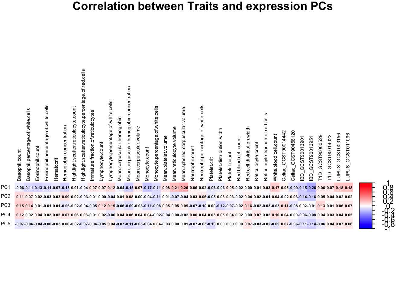
Artery Aorta Validation

Correlation between PRS & expression PCs

# load prs & pcs
metadata_file <- "analysis/metadata_artery.txt"
metadata <- read.csv(metadata_file, header = T, sep = "\t", stringsAsFactors = T)
metadata$sex <- as.factor(metadata$sex)

traits <- metadata[, 7:43]
pc <- metadata[, 1:5]

# Calculate the correlation between each trait and each PC
correlation_matrix <- cor(traits, pc)
range(correlation_matrix)

[1] -0.2613287  0.2585593

correlation_matrix <- t(correlation_matrix)

# Create the heatmap using corrplot
corrplot(correlation_matrix, method = "color", 
         col = colorRampPalette(c("blue", "white", "red"))(200), # color palette
         addCoef.col = "black", # Add correlation coefficients to the plot
         number.cex = 0.4, # Adjust the font size of the numbers
         tl.col = "black", # text label color
         tl.srt = 90, # rotate text labels
         tl.cex = 0.5, 
         title = "Correlation between Traits and expression PCs", 
         mar = c(0, 0, 1, 0)
)

Past versions of unnamed-chunk-1-1.png

Version	Author	Date
8aa2b83	ElisaChen	2025-05-14

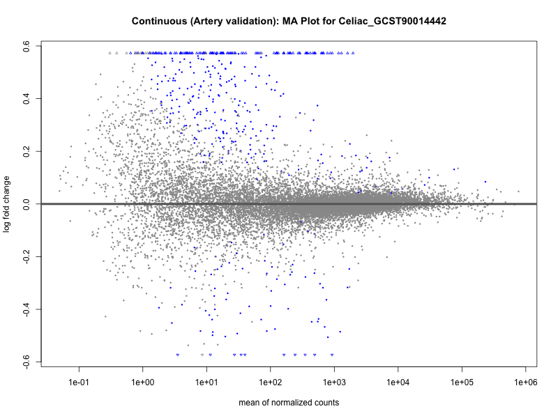
Perform DESeq2 differential expression analysis for each trait

# Load the gene expression data
gene_expr_file <- "data/gene_reads_2017-06-05_v8_artery_aorta.gct"
raw_count_df <- fread(gene_expr_file, header = TRUE, sep = "\t", drop = "id")

# load protein_coding list
protein_coding <- fread("data/protein-coding_gene.txt", sep = "\t")
protein_coding <- protein_coding[, c("symbol", "ensembl_gene_id")]

# keep only protein-coding genes
raw_count_df <- raw_count_df[raw_count_df$Description %in% protein_coding$symbol, ]

id <- raw_count_df$Name
raw_count <- raw_count_df[, -c(1:2)]

# modify GTEx sample names matching names used in PRS data
colnames(raw_count) <- sub("^(GTEX-[^-.]+).*", "\\1", colnames(raw_count))

matching_samples <- intersect(rownames(metadata), colnames(raw_count))
final_count <- raw_count[ , ..matching_samples]

# prefilter: keep only rows that have a count of at least 10
keep_genes <- rowSums(final_count >= 10) > 0
final_count <- final_count[keep_genes, ]
id <- id[keep_genes]
dim(final_count)

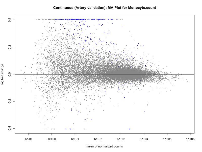
# Loop through each trait and run DESeq2
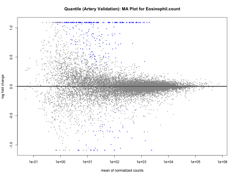
for (trait in colnames(traits)) {
  
  # Standardize PRS for the current trait
  prs_trait <- traits[,trait]
  prs_trait <- scale(prs_trait) # Standardize PRS to mean = 0, sd = 1
    
  # Add the standardized PRS to the metadata for continuous trait
  metadata[,trait] <- prs_trait
  
  # Create the DESeqDataSet for the current trait
  dds <- DESeqDataSetFromMatrix(
    countData = as.matrix(final_count),  # Raw counts
    colData = metadata[, c(1:6, which(colnames(metadata) == trait))],
    design = as.formula(paste("~ PC1 + PC2 + PC3 + PC4 + PC5 + sex +", trait))
  )
  rownames(dds) <- id
  
  # Run DESeq2 analysis
  dds <- DESeq(dds, parallel = TRUE, BPPARAM = MulticoreParam(4))
  
  # Get the results for the current trait
  res <- results(dds)
  
  # Save the results to a file
  write.csv(res, paste0("validation_", trait, "_results_artery_validation.csv"))
  
  # print a summary of the results
  print(paste("Results for trait:", trait))
  print(summary(res))
  
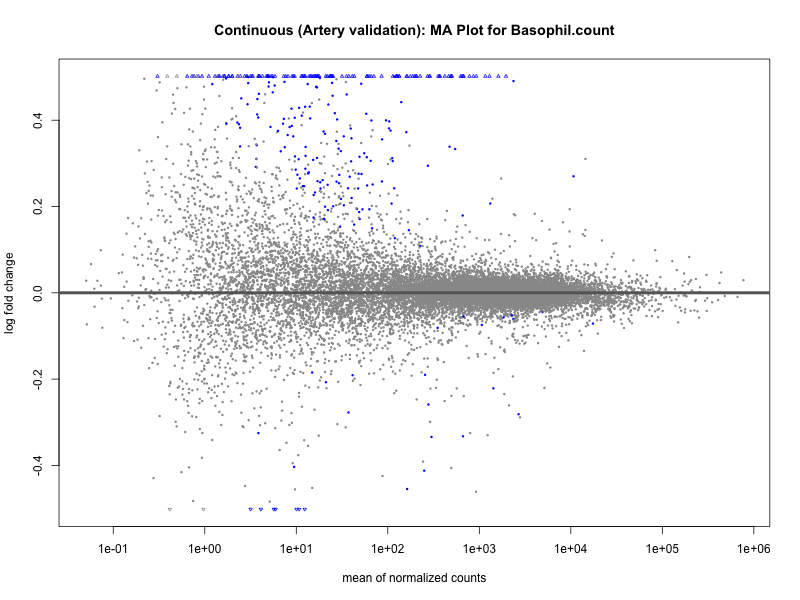
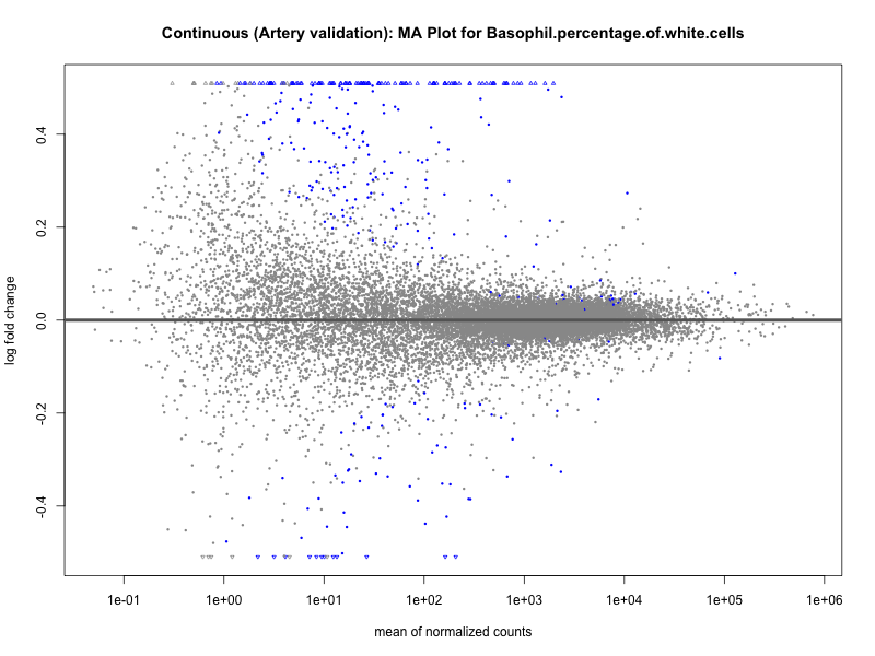
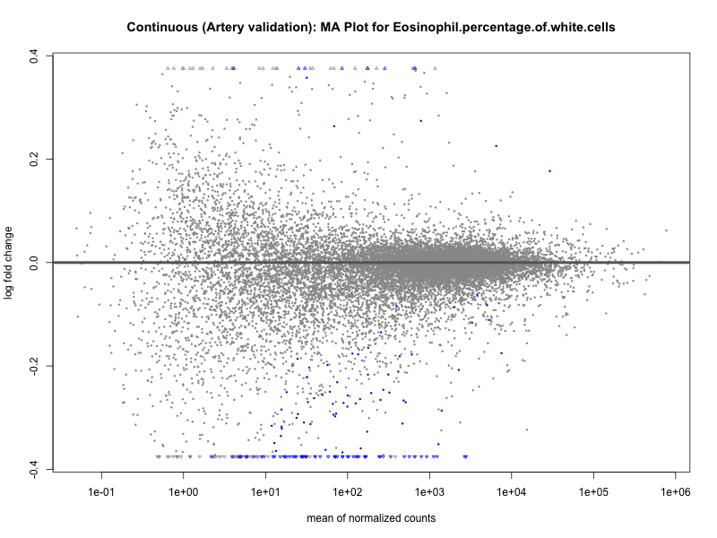
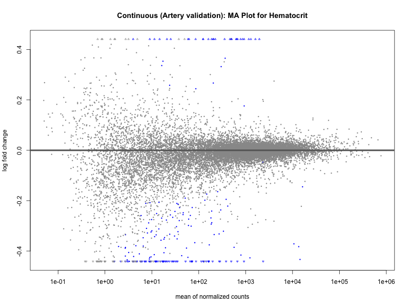
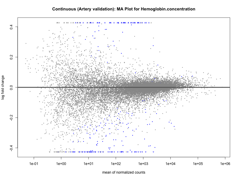
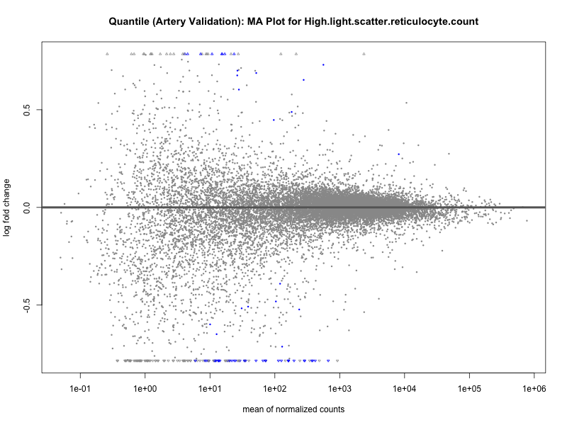
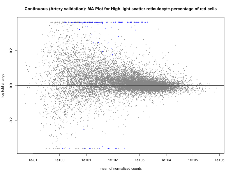
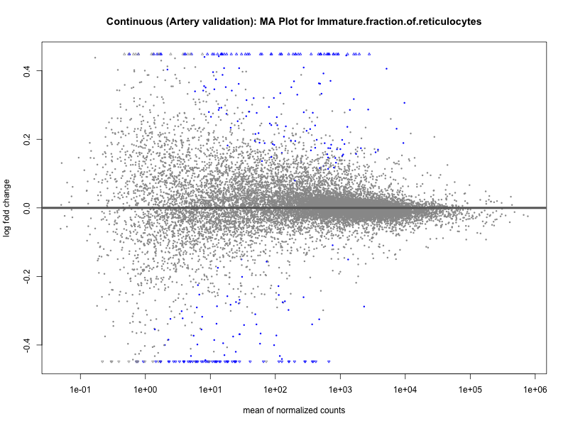
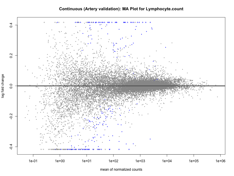
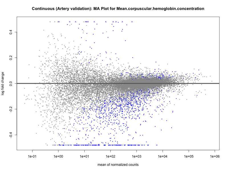
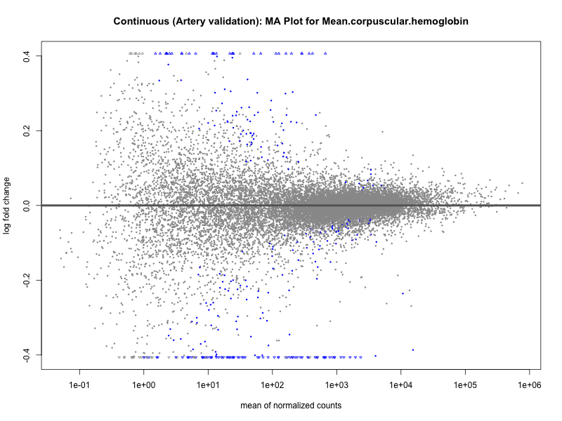
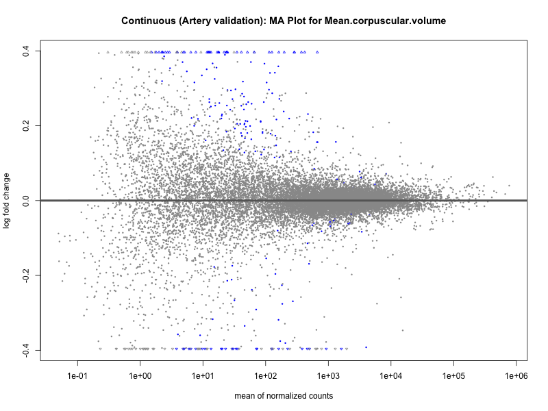
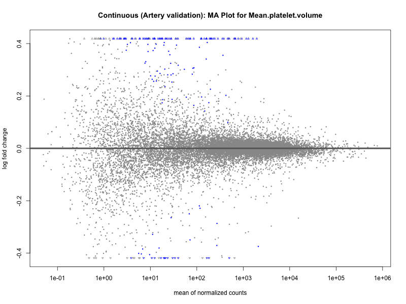
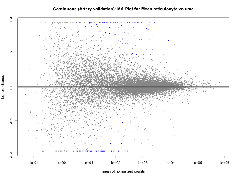
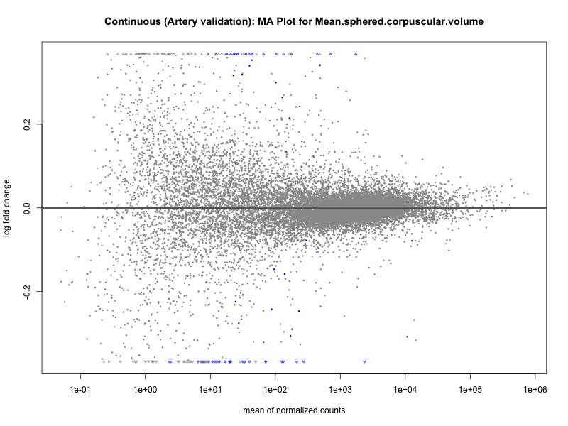
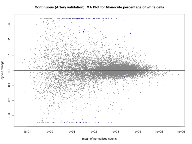
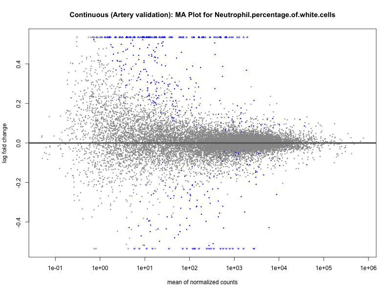
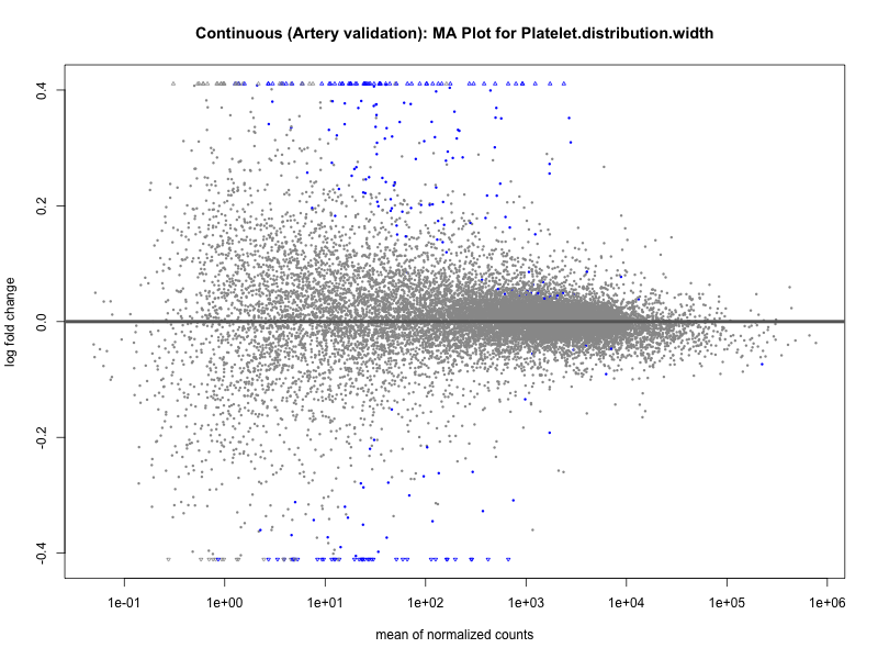
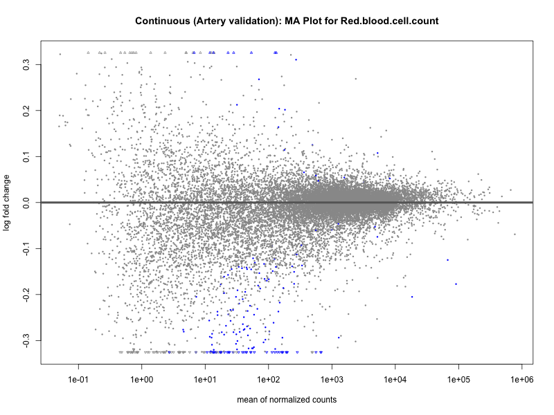
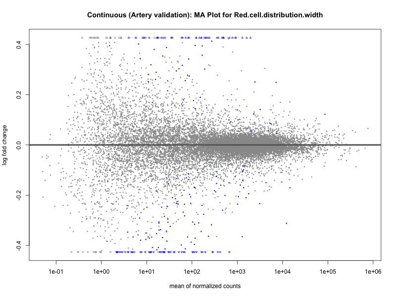
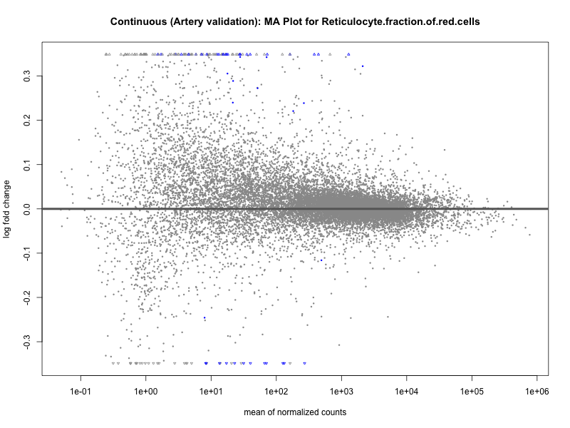
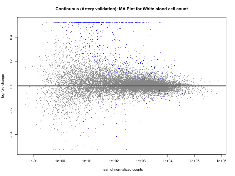
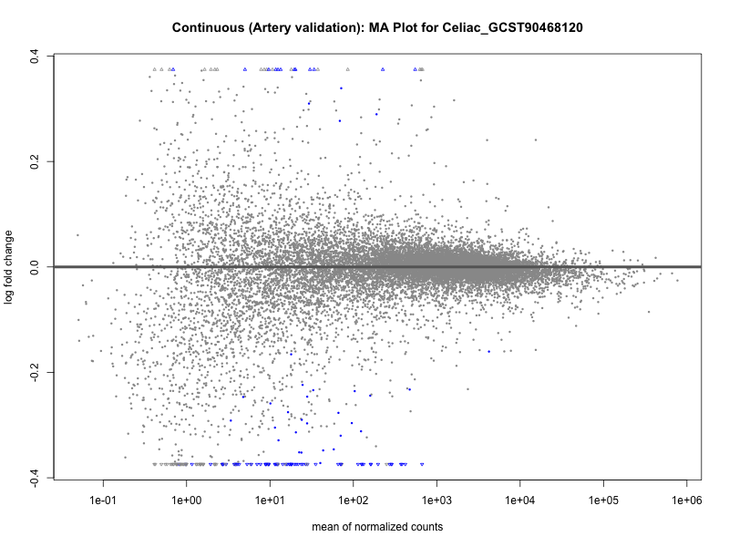
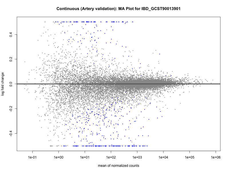
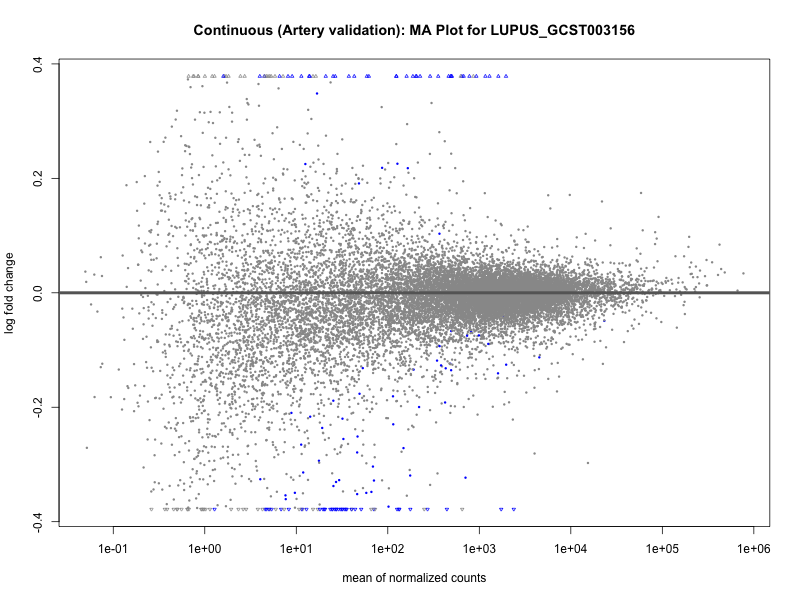
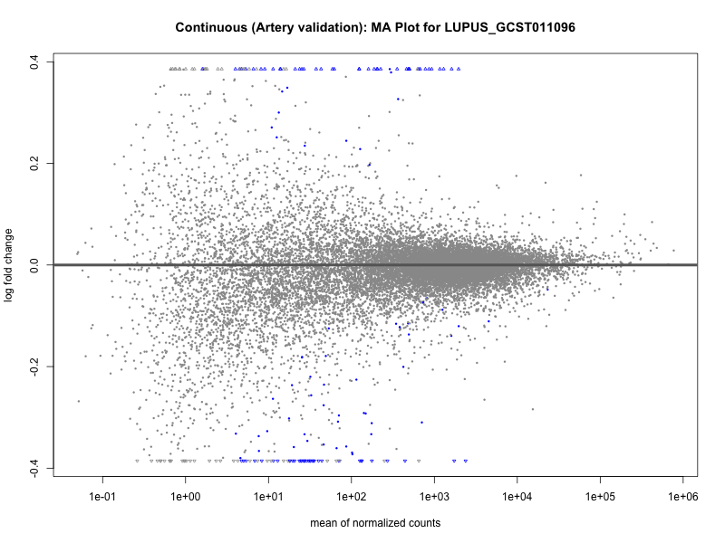
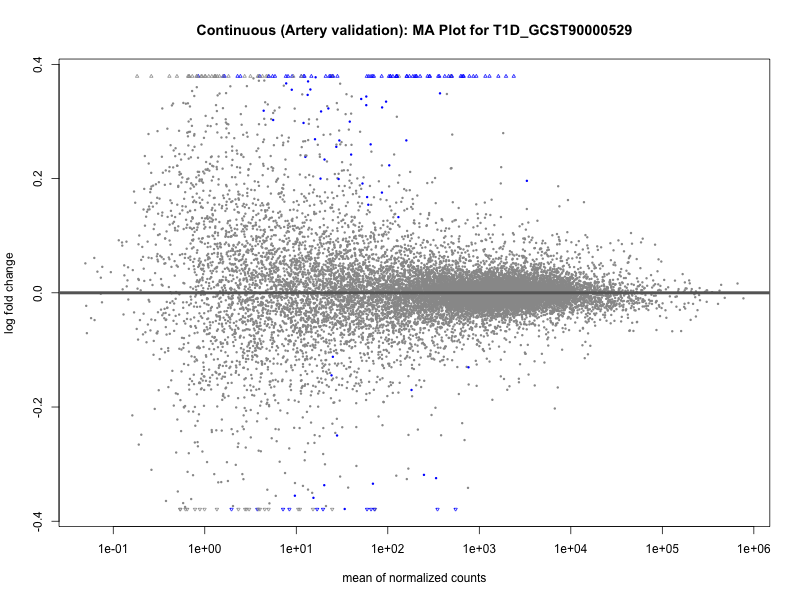
  # plot the MA-plot for the current trait
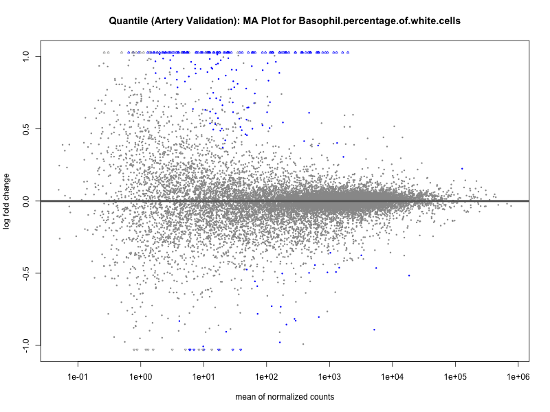
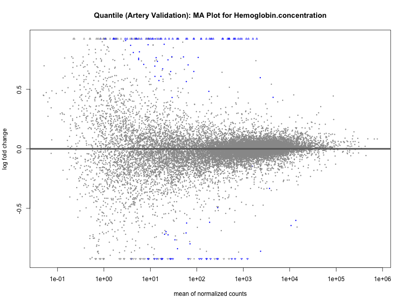
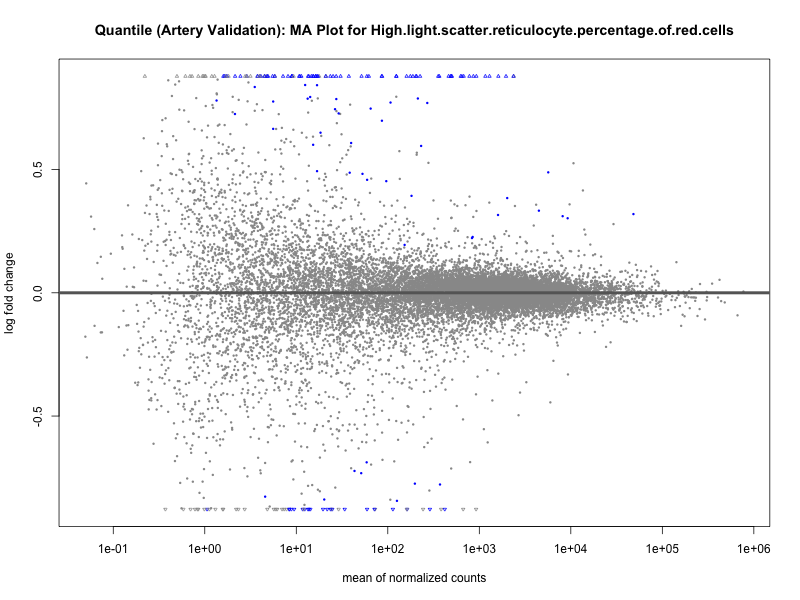
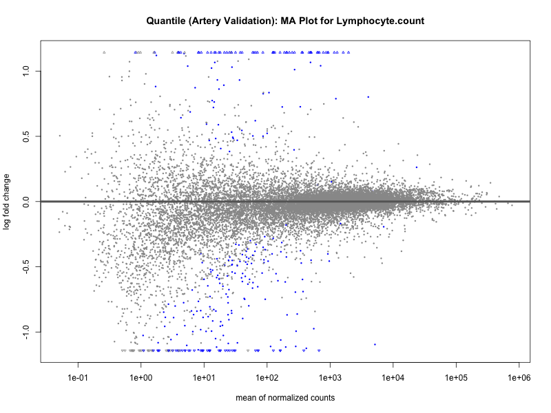
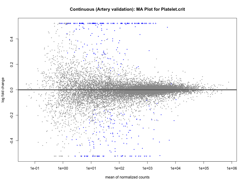
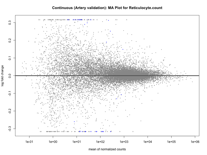
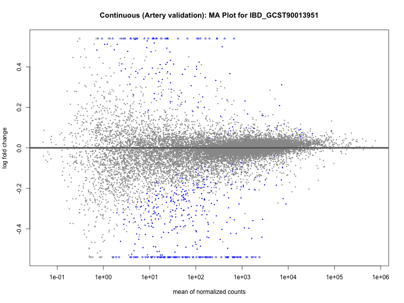
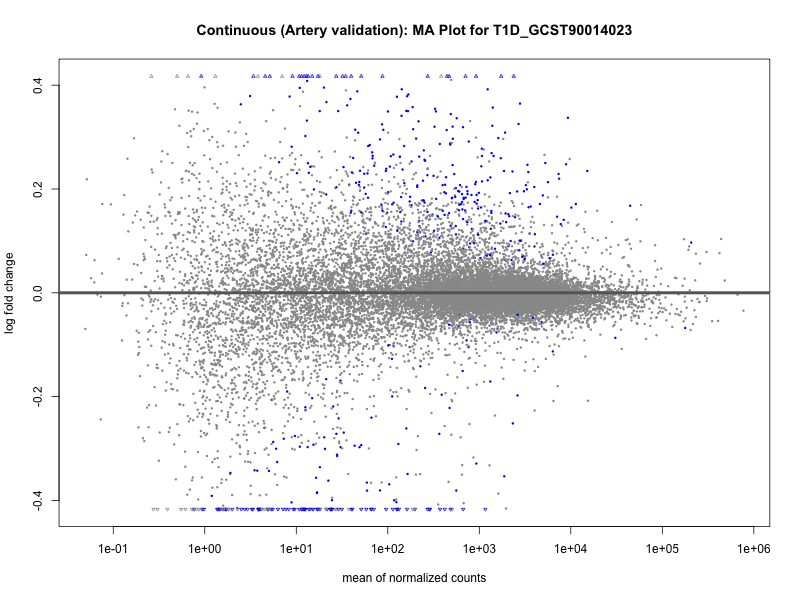
  png(paste0("ma_plot_", trait, "_artery_validation.png"), width = 800, height = 600)
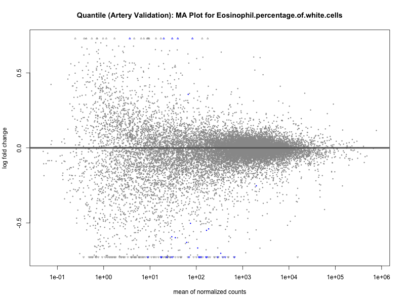
  plotMA(res, main = paste("Continuous (Artery validation): MA Plot for", trait))
  dev.off()
  
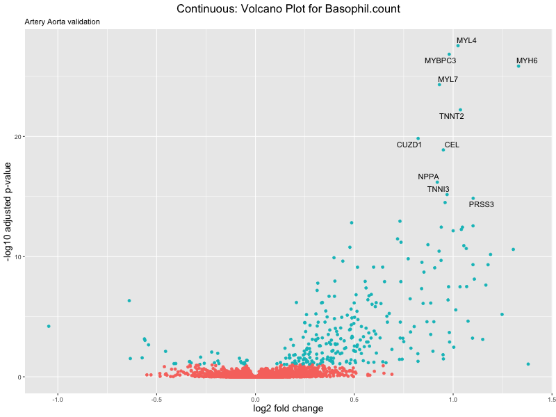
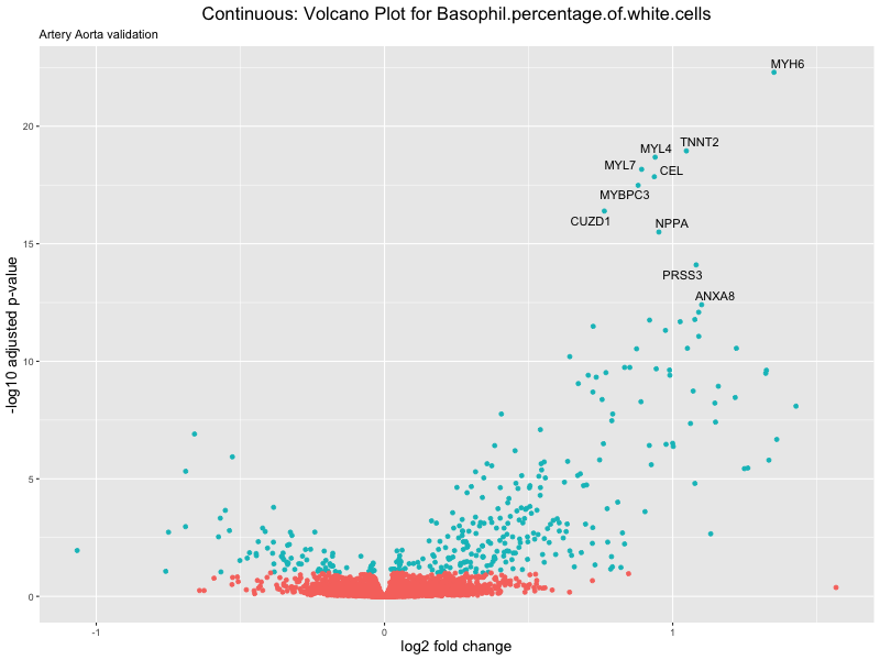
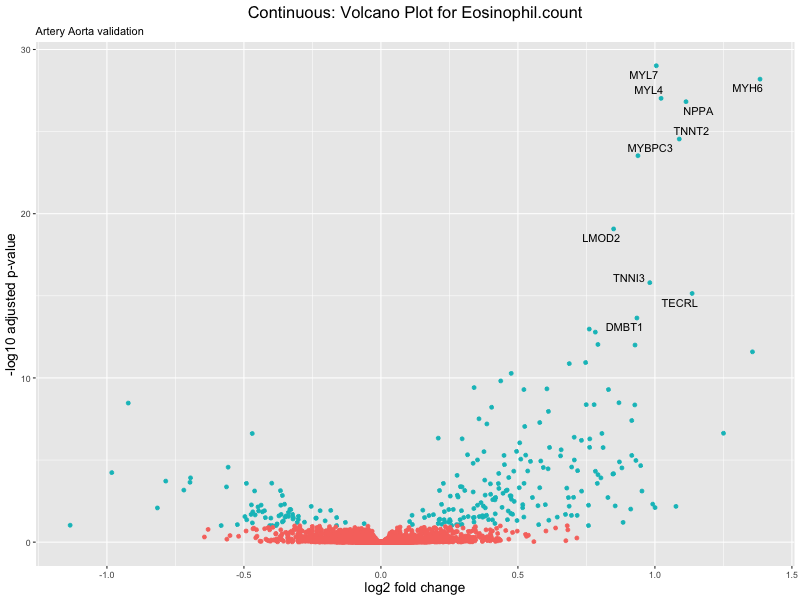
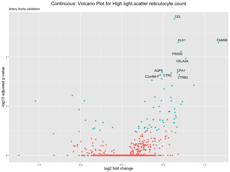
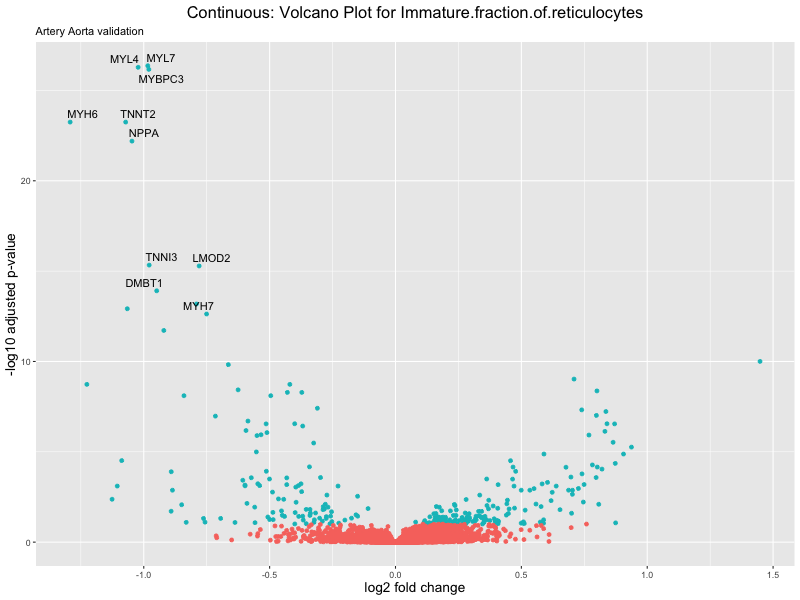
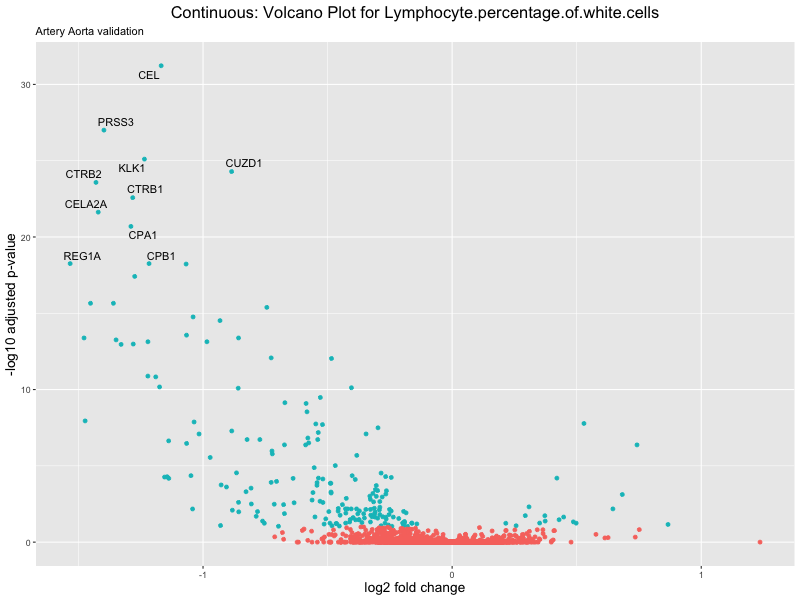
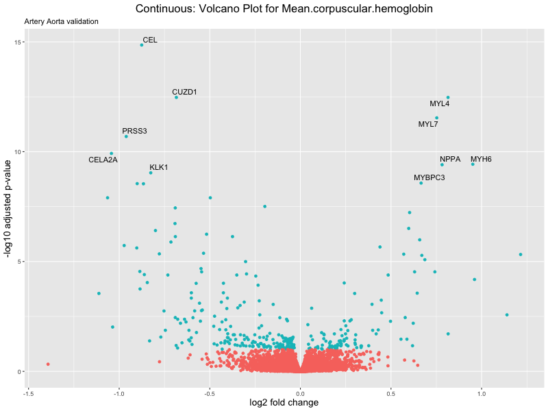
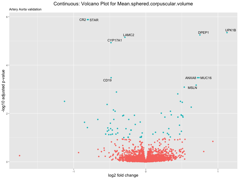
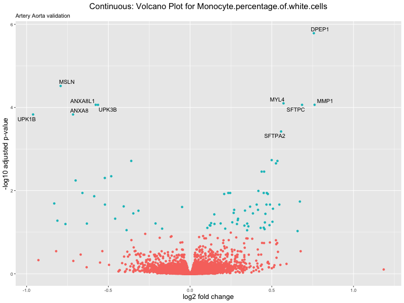
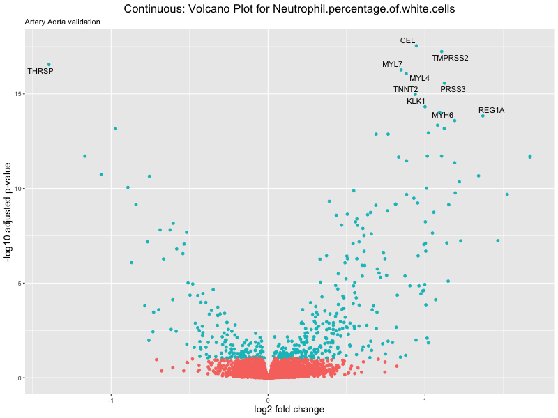
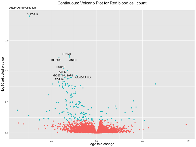
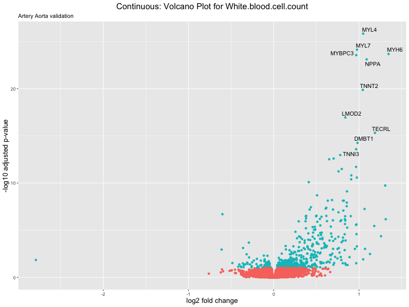
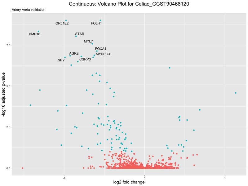
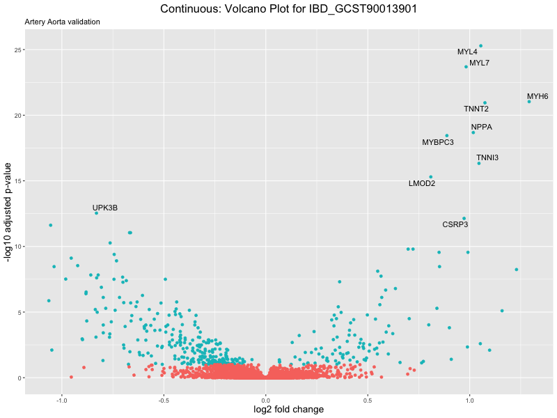
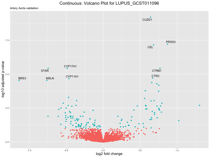
  # volcano plot
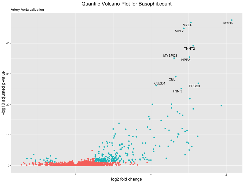
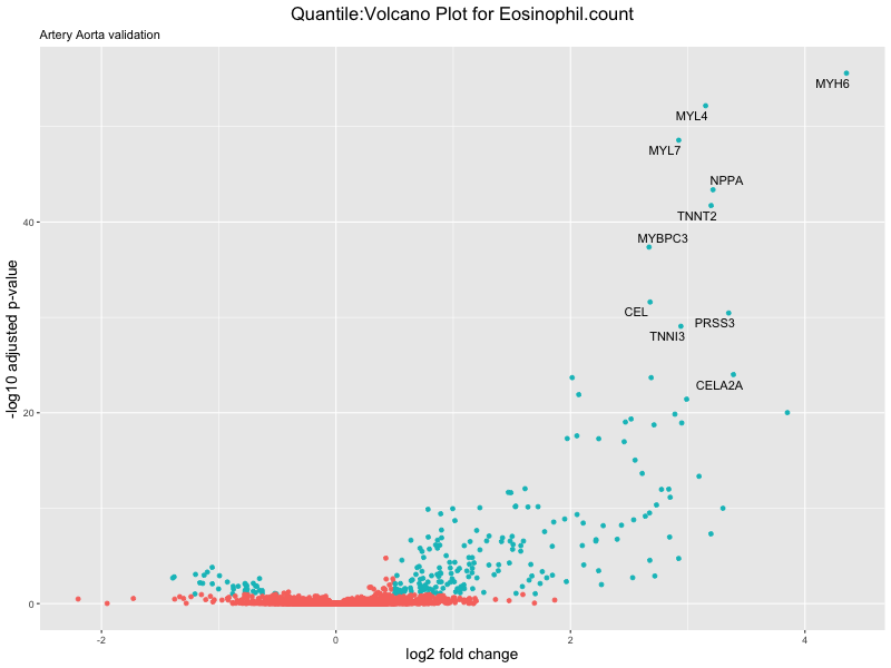
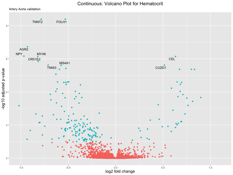
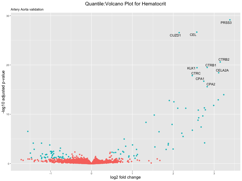
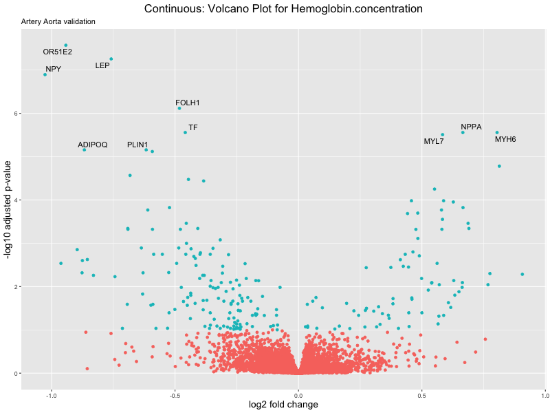
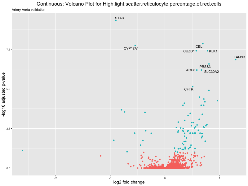
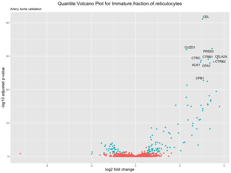
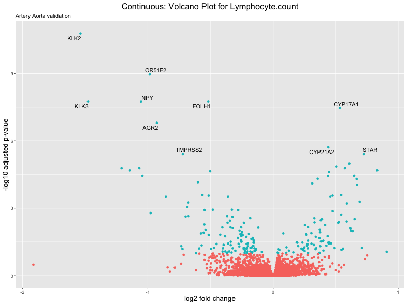
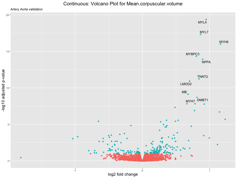
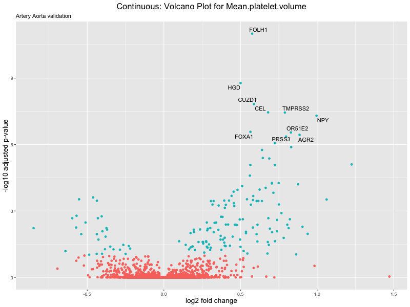
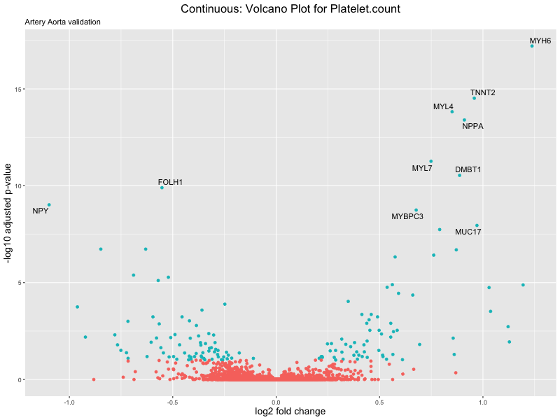
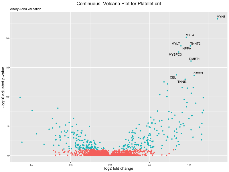
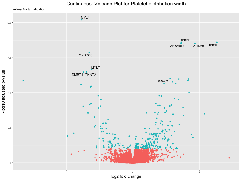
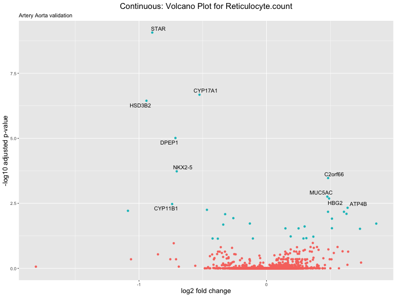
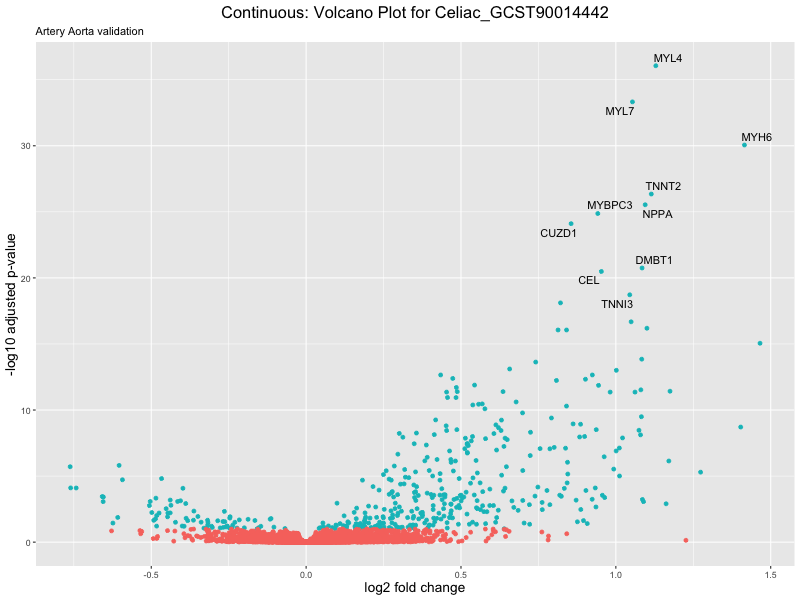
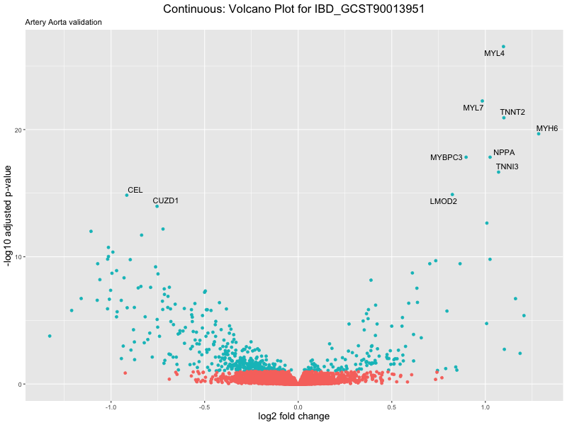
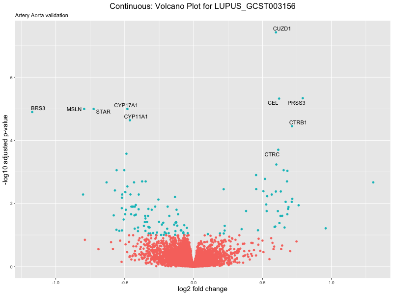
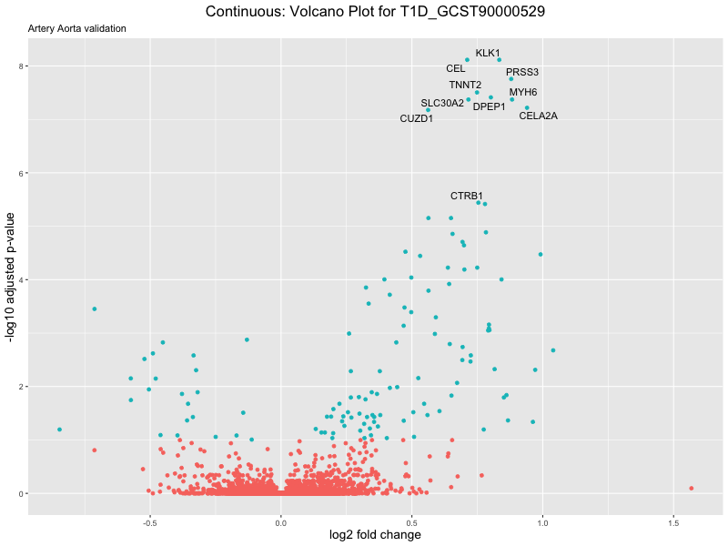
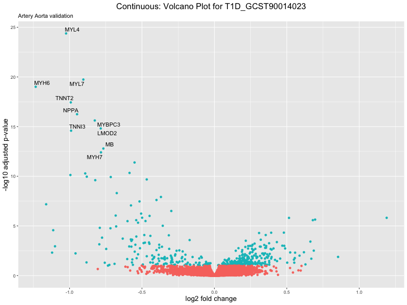
  res_tableOE <- as.data.frame(res)
  res_tableOE$gene_name <- raw_count_df$Description[keep_genes]
  res_tableOE <- mutate(res_tableOE, threshold_OE = padj < 0.1)
  res_tableOE <- res_tableOE %>% arrange(padj) %>% mutate(genelabels = "")
  res_tableOE$genelabels[1:10] <- res_tableOE$gene_name[1:10]
  
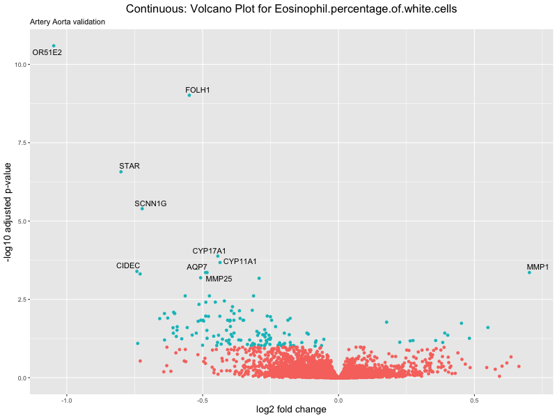
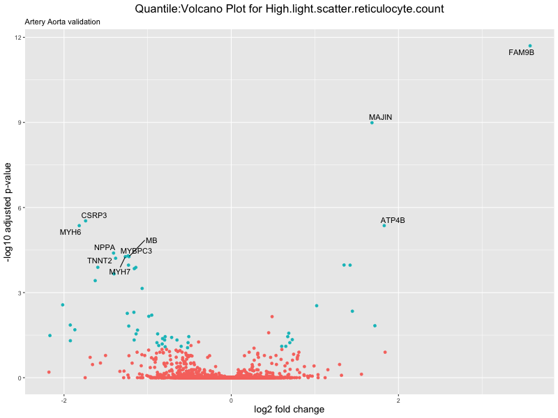
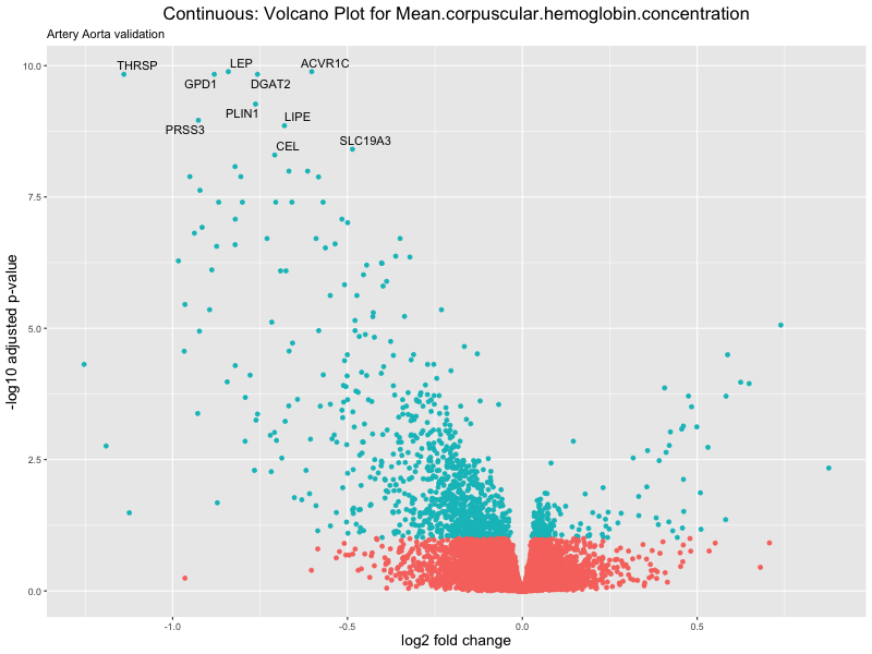
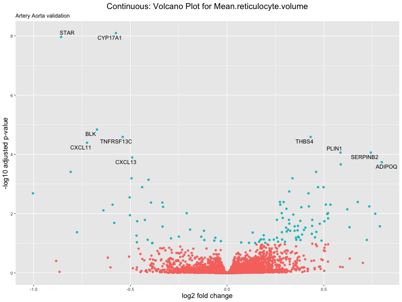
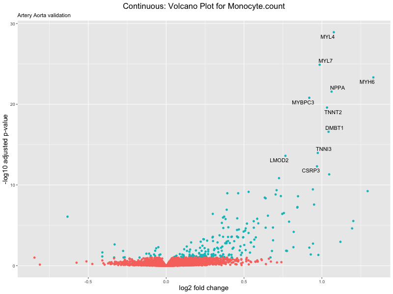
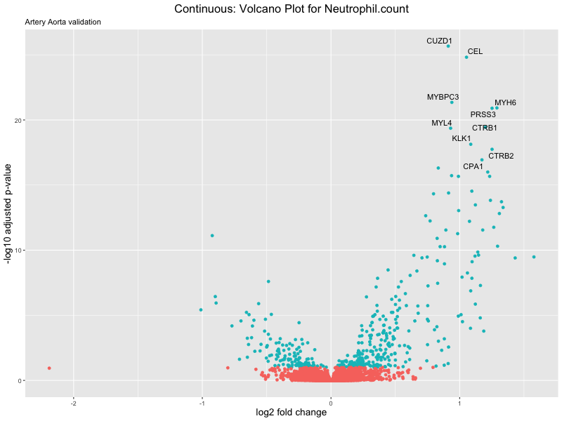
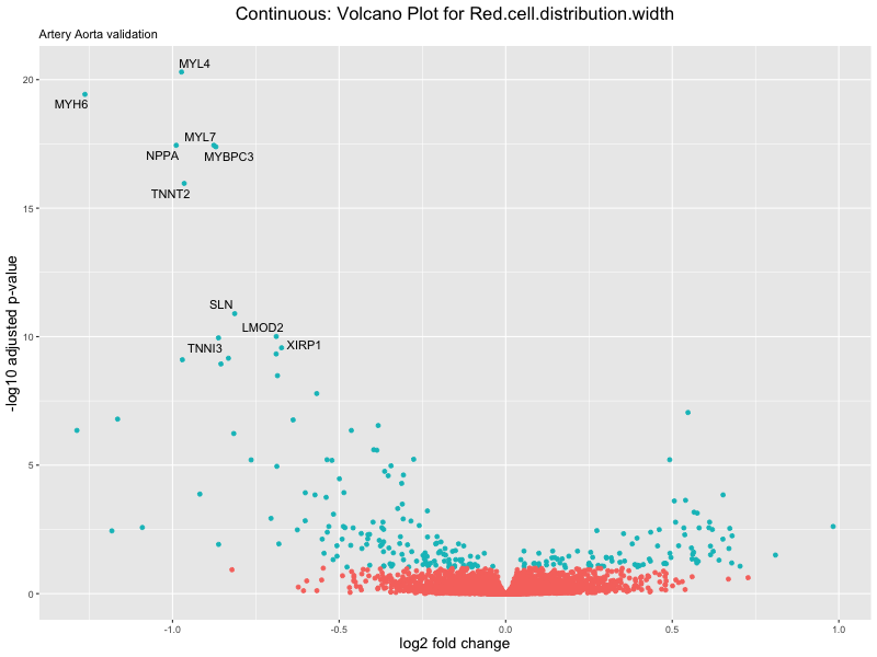
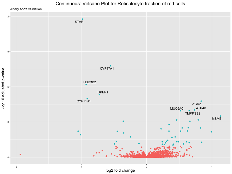
  volcano_plot <- ggplot(res_tableOE, aes(x = log2FoldChange, y = -log10(padj))) +
    geom_point(aes(colour = threshold_OE)) +
    geom_text_repel(aes(label = genelabels)) +
    ggtitle(label = paste("Continuous: Volcano Plot for", trait), 
            subtitle = "Artery Aorta validation") +
    xlab("log2 fold change") + 
    ylab("-log10 adjusted p-value") +
    theme(legend.position = "none",
          plot.title = element_text(size = rel(1.5), hjust = 0.5),
          axis.title = element_text(size = rel(1.25)))
  
  # Save the volcano plot
  png(paste0("volcano_plot_", trait, "_artery_validation.png"), width = 800, 
      height = 600)
  print(volcano_plot)
  dev.off()
}

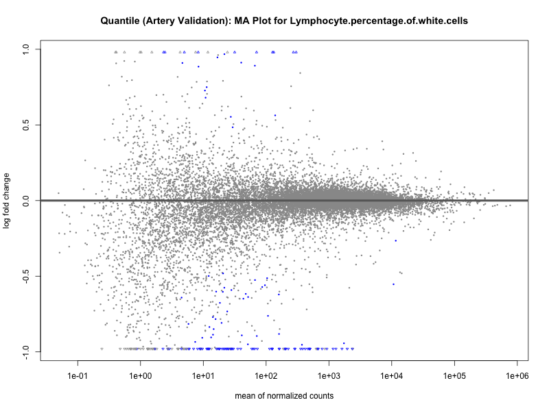
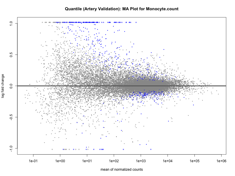
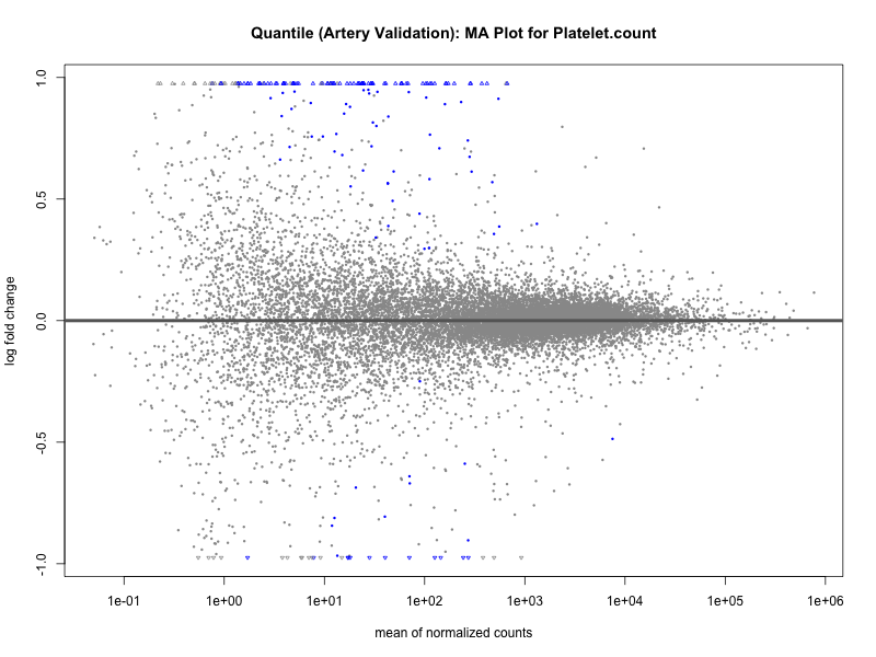
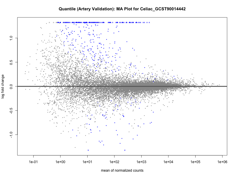
metadata_file <- "analysis/metadata_artery_quantile.txt"
metadata <- read.csv(metadata_file, header = T, sep = "\t", stringsAsFactors = T)
metadata$sex <- as.factor(metadata$sex)

traits <- metadata[, 7:43]

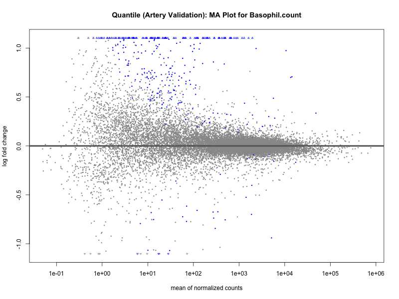
# Loop through each trait and run DESeq2
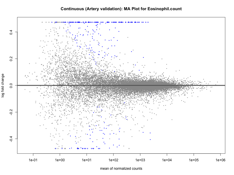
for (trait in colnames(traits)) {
  
  # Create the DESeqDataSet for the current trait
  dds <- DESeqDataSetFromMatrix(
    countData = as.matrix(final_count),  # Raw counts
    colData = metadata[, c(1:6, which(colnames(metadata) == trait))],
    design = as.formula(paste("~ PC1 + PC2 + PC3 + PC4 + PC5 + sex +", trait))
  )
  rownames(dds) <- id
  
  # Run DESeq2 analysis
  dds <- DESeq(dds, parallel = TRUE, BPPARAM = MulticoreParam(4))
  
  # Get the results for the current trait
  res <- results(dds)
  
  # Save the results to a file
  write.csv(res, paste0("validation_", trait, "_quantile_results_artery_validation.csv"))
  
  # print a summary of the results
  print(paste("Results for trait:", trait))
  print(summary(res))
  
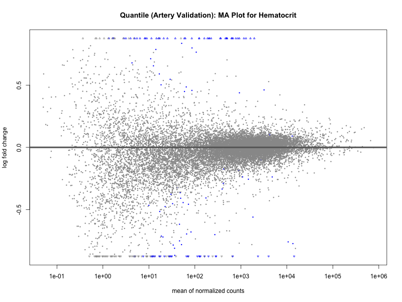
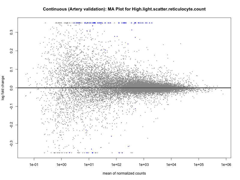
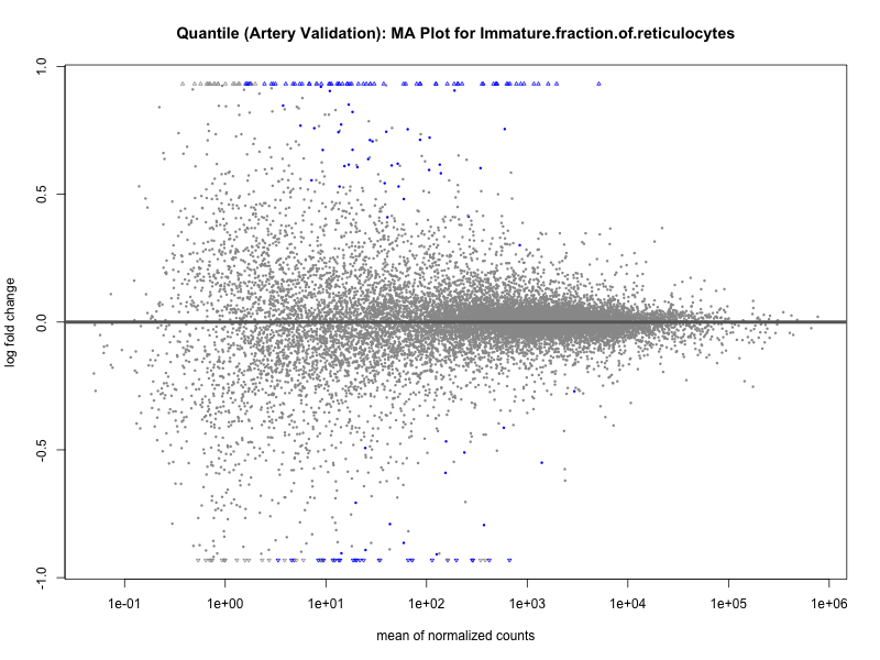
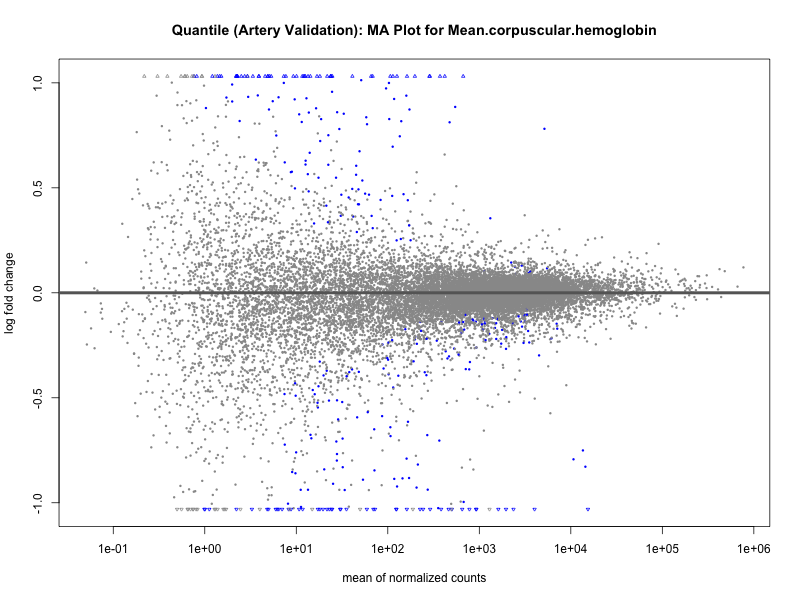
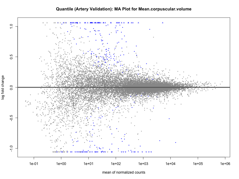
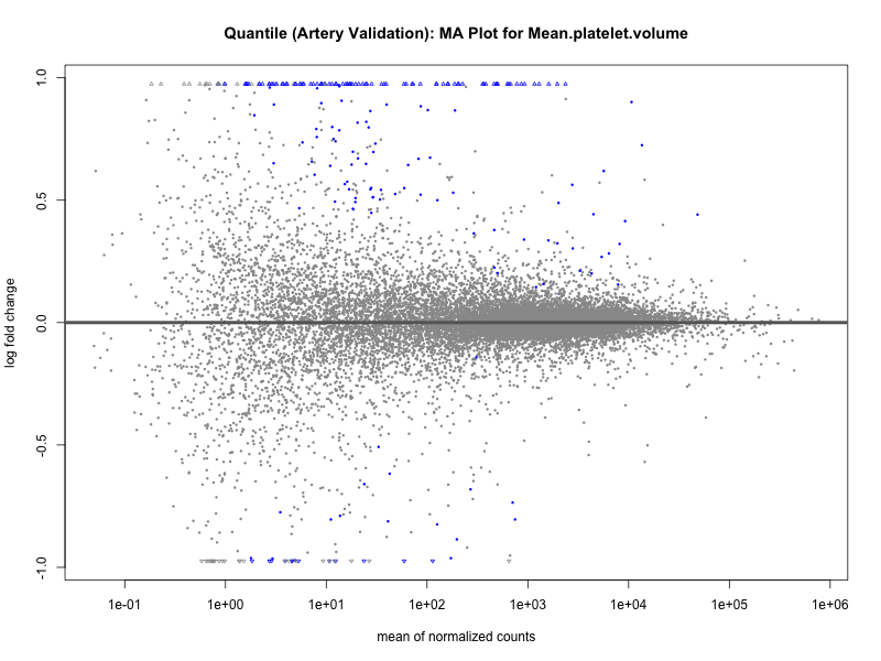
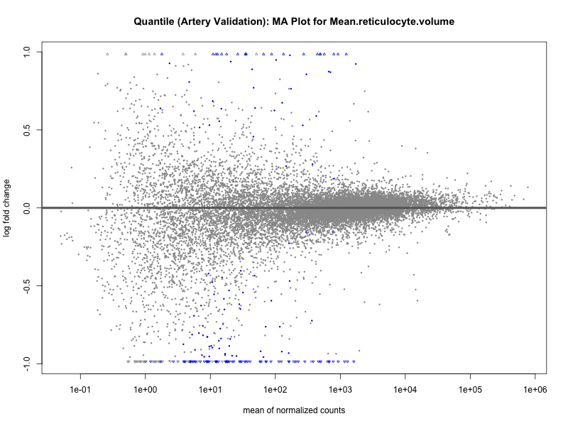
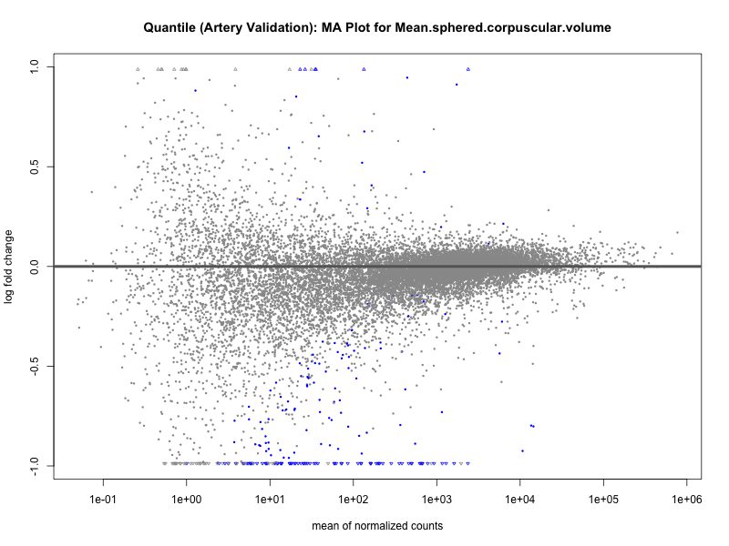
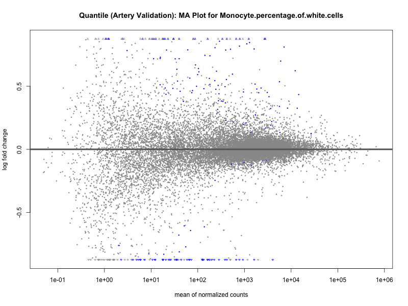
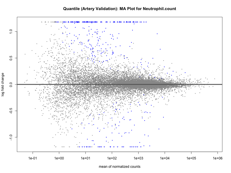
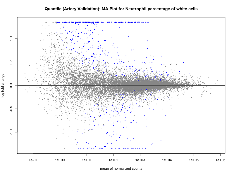
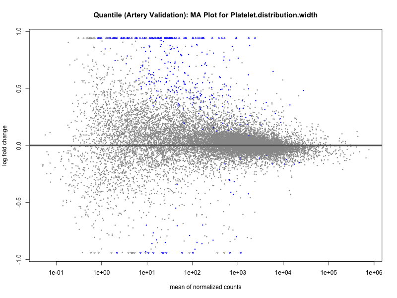
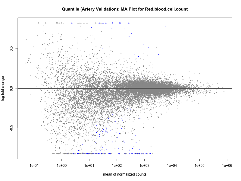
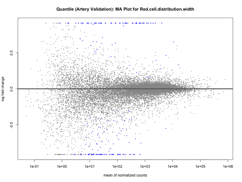
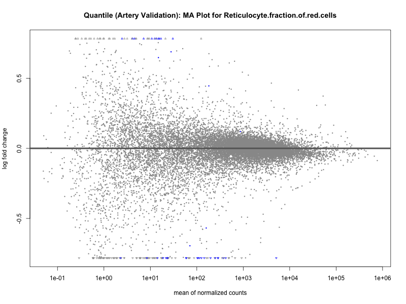
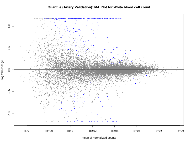
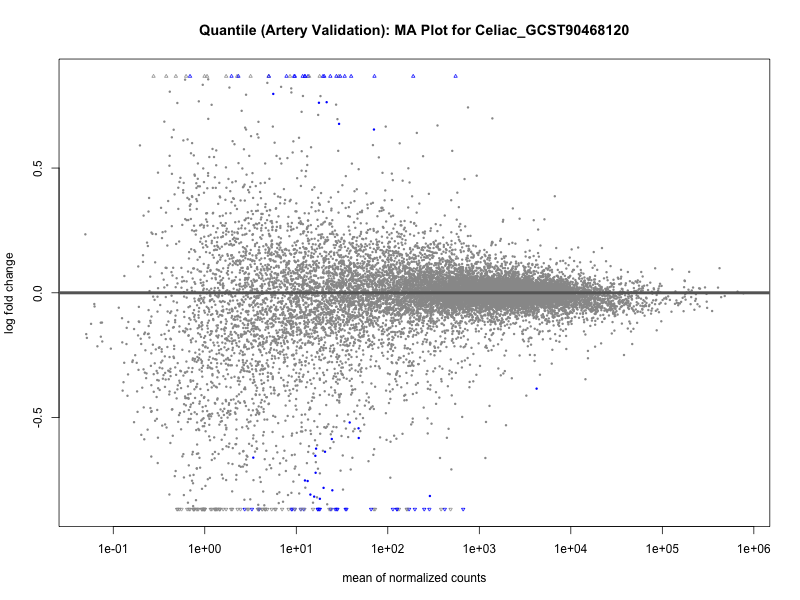
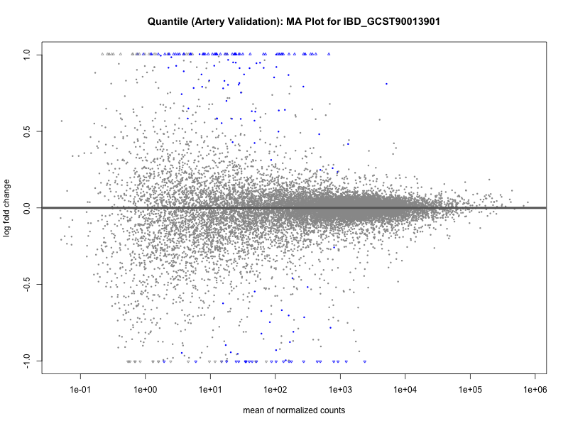
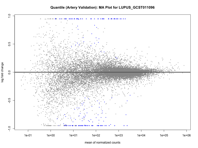
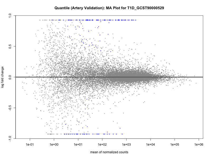
  # plot the MA-plot for the current trait
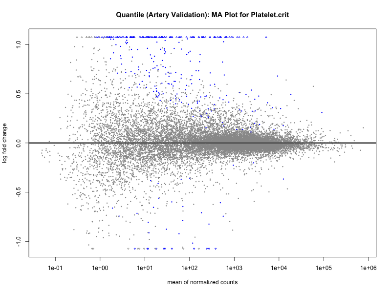
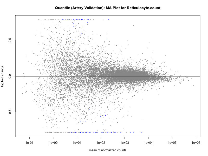
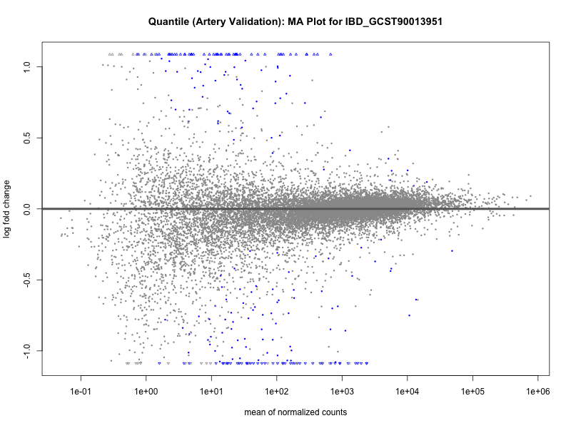
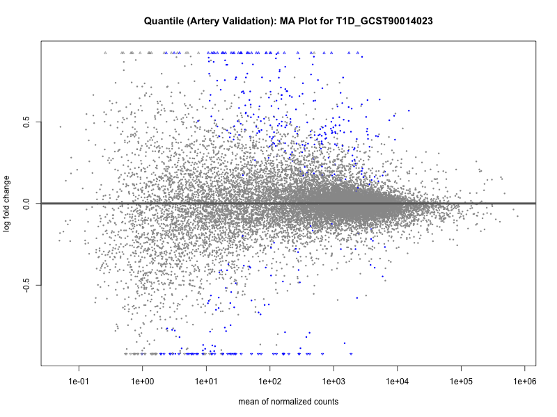
  png(paste0("ma_plot_quantile_", trait, "_artery_validation.png"), width = 800, height = 600)
  plotMA(res, main = paste("Quantile (Artery Validation): MA Plot for", trait))
  dev.off()
  
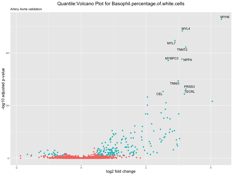
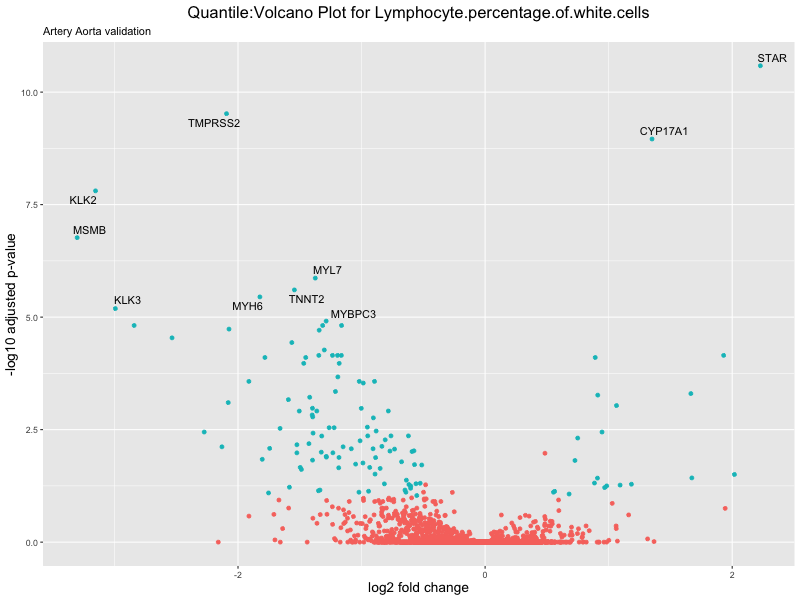
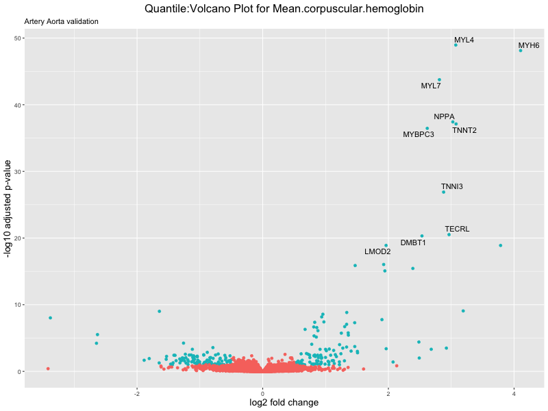
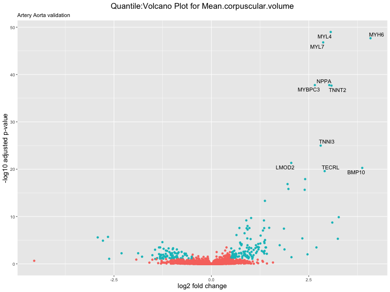
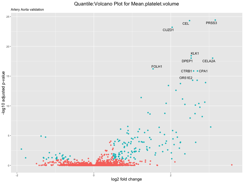
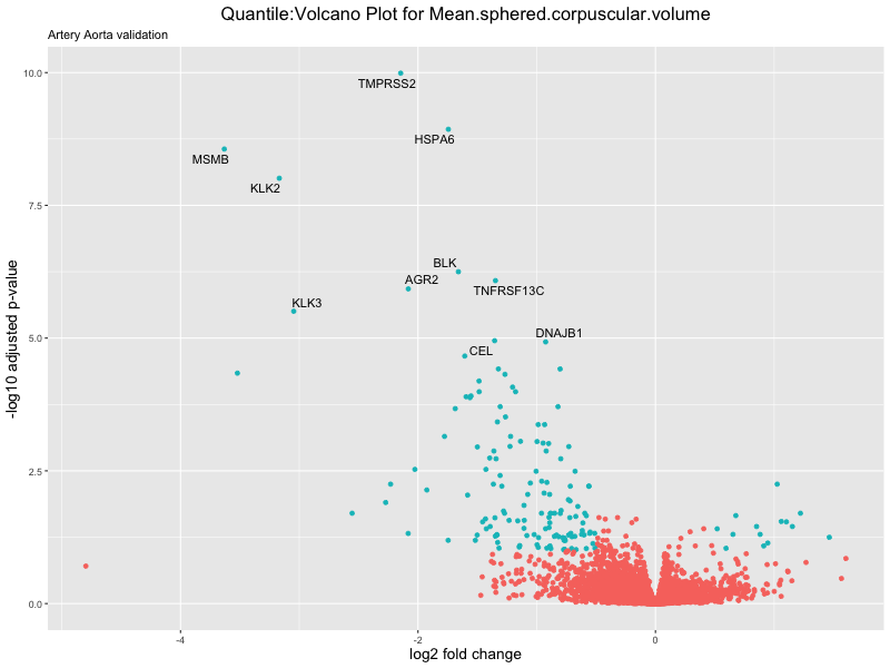
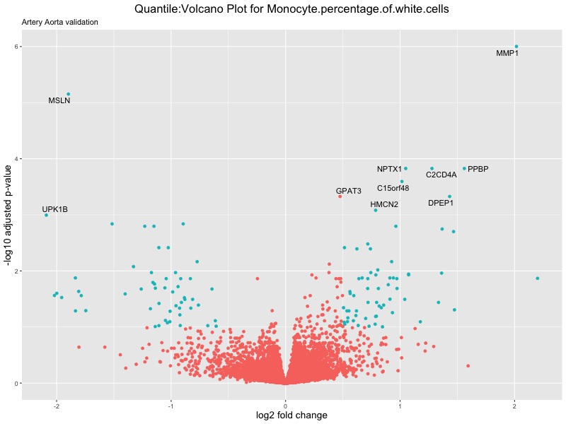
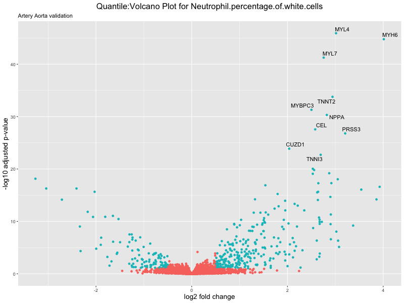
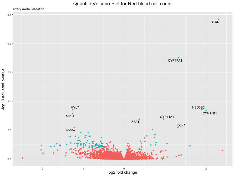
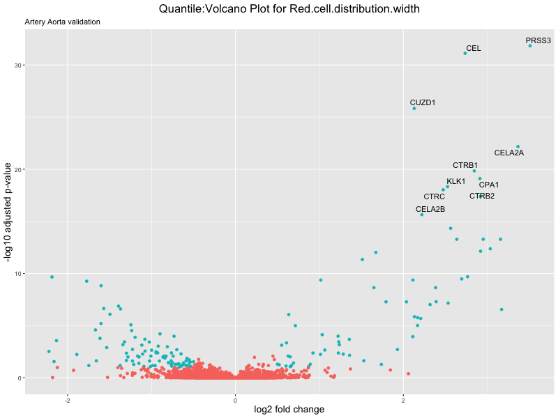
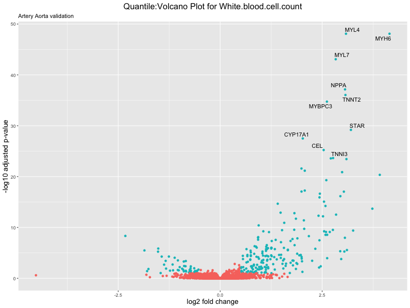
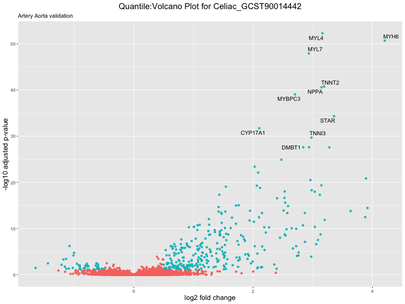
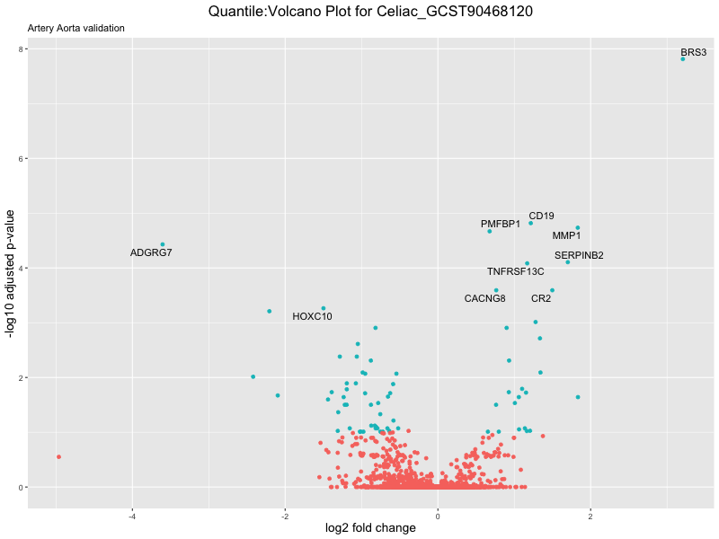
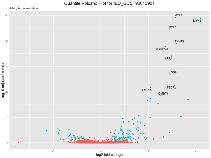
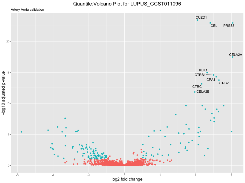
  # volcano plot
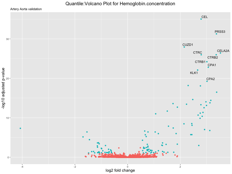
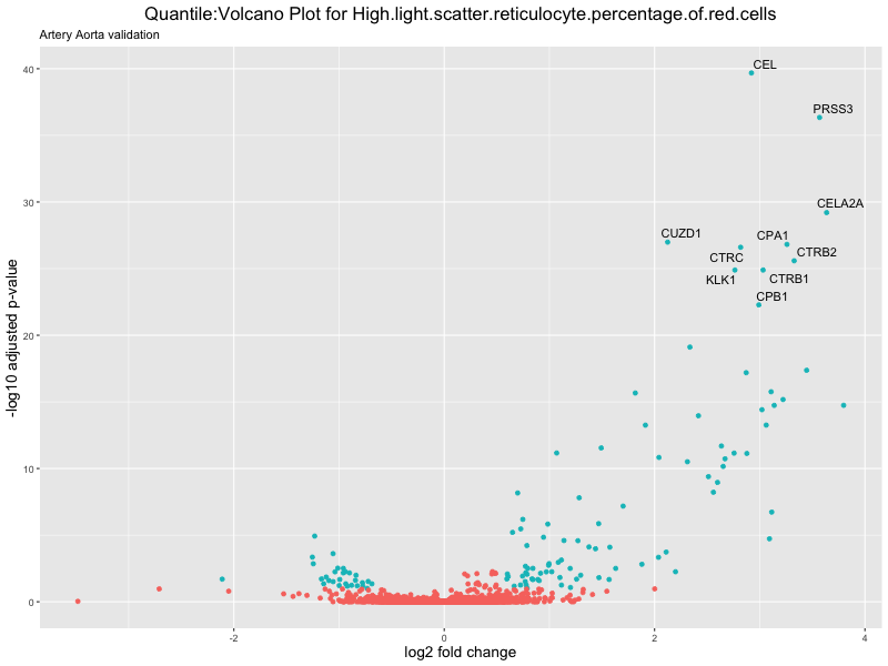
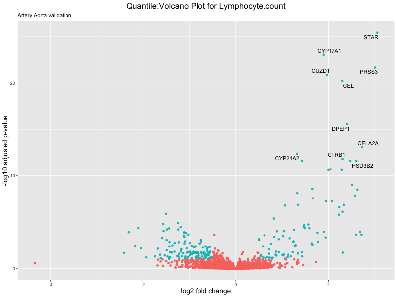
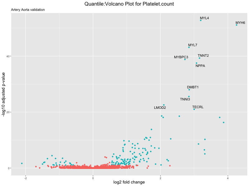
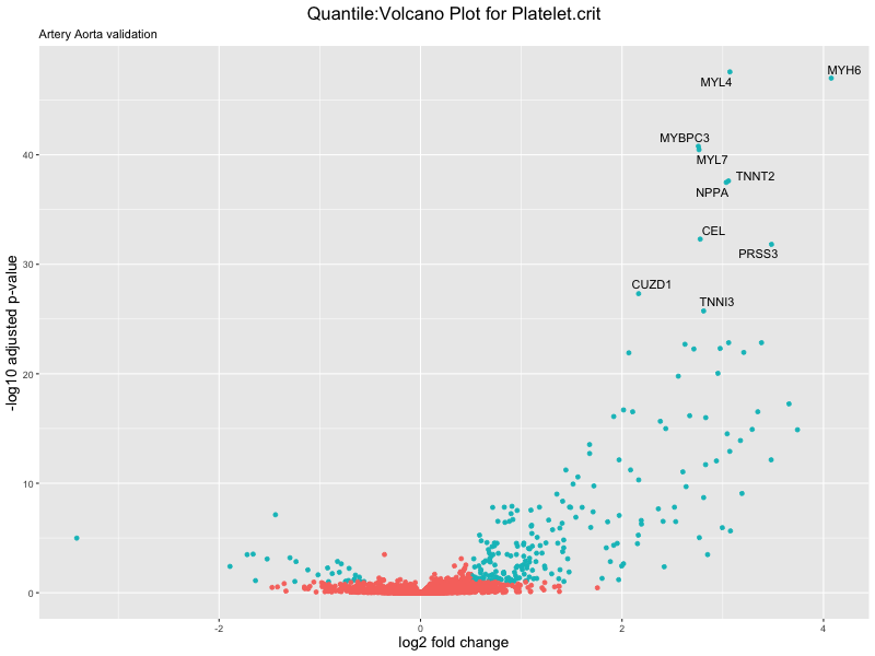
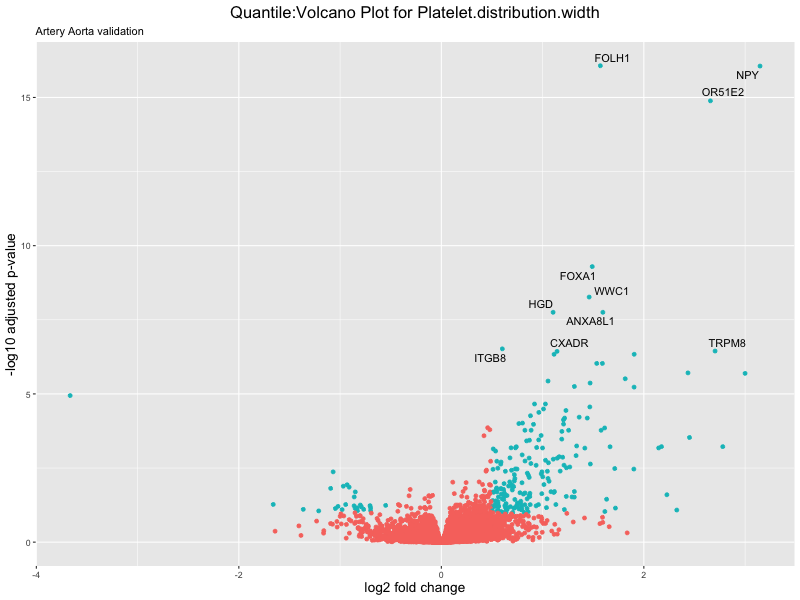
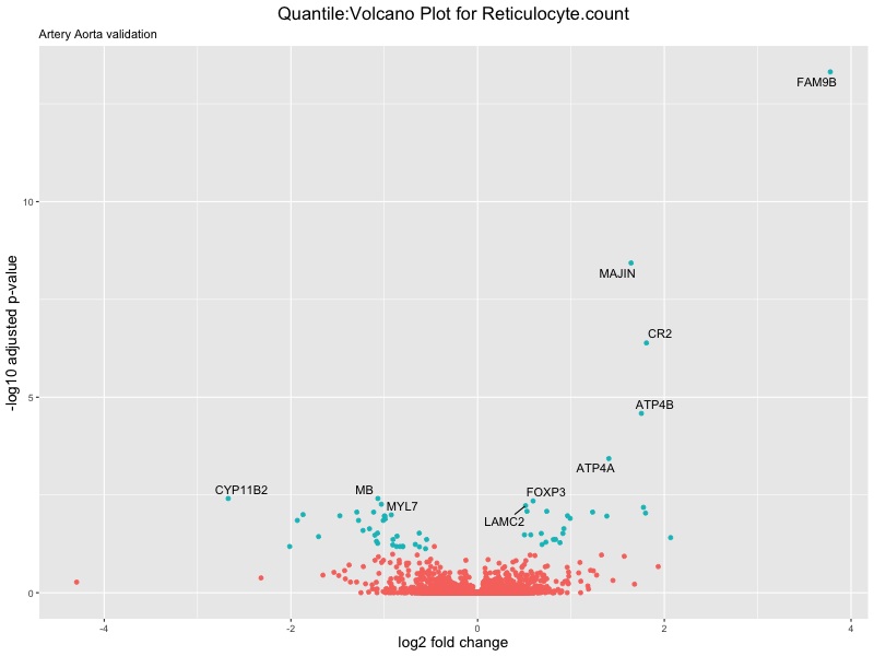
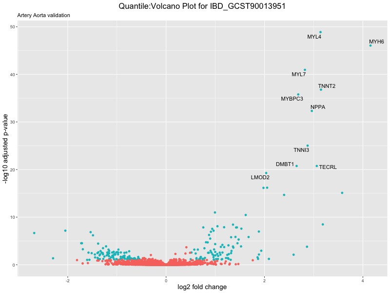
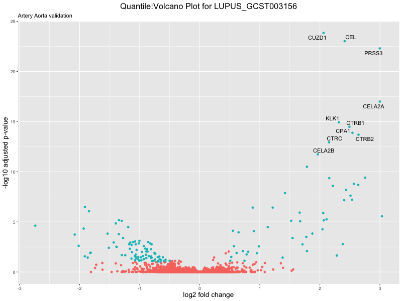
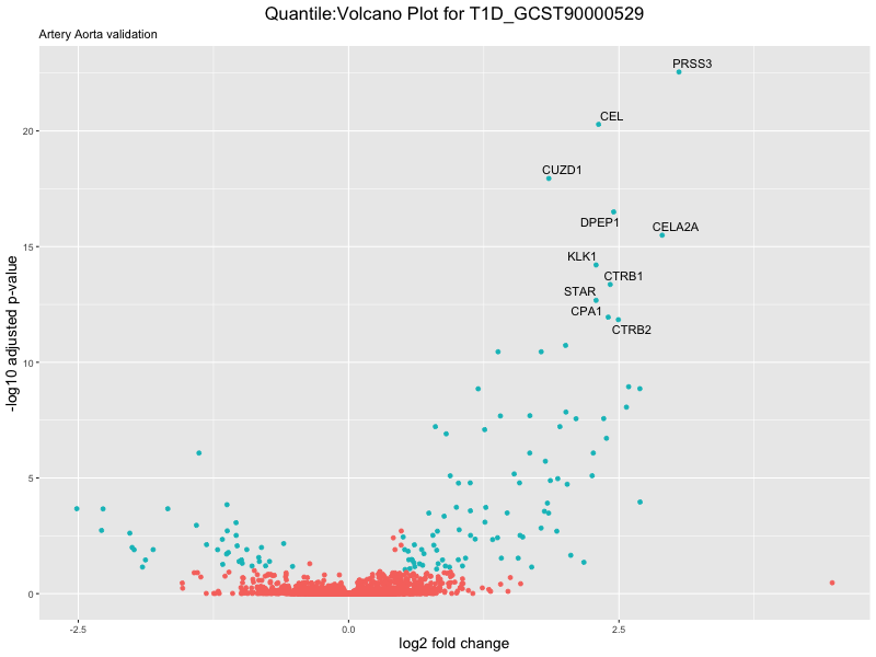
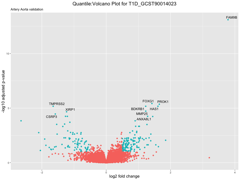
  res_tableOE <- as.data.frame(res)
  res_tableOE$gene_name <- raw_count_df$Description[keep_genes]
  res_tableOE <- mutate(res_tableOE, threshold_OE = padj < 0.1 & 
                          abs(log2FoldChange) >= 0.5)
  res_tableOE <- res_tableOE %>% arrange(padj) %>% mutate(genelabels = "")
  res_tableOE$genelabels[1:10] <- res_tableOE$gene_name[1:10]
  
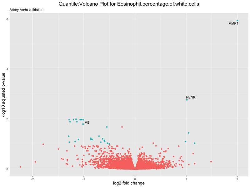
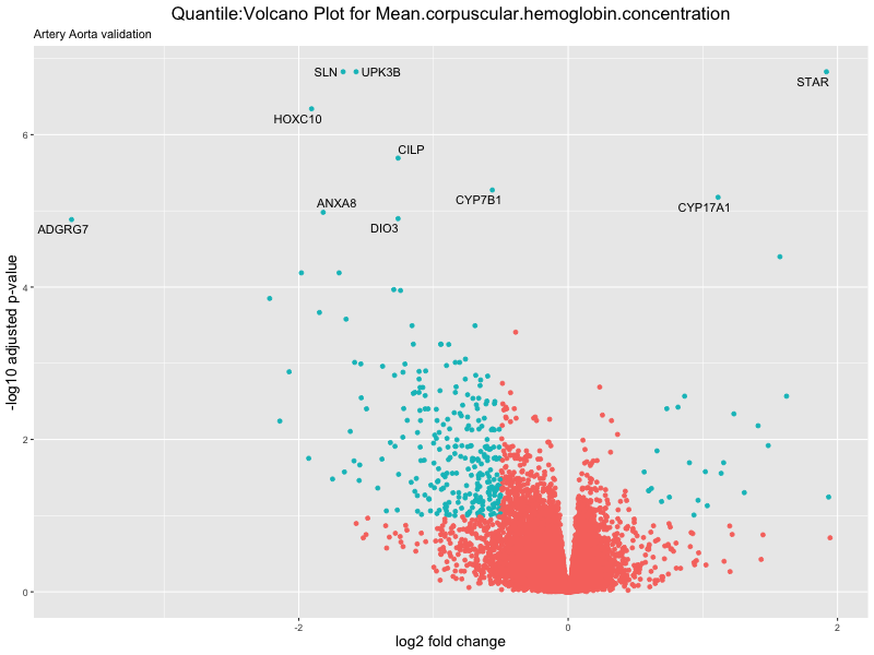
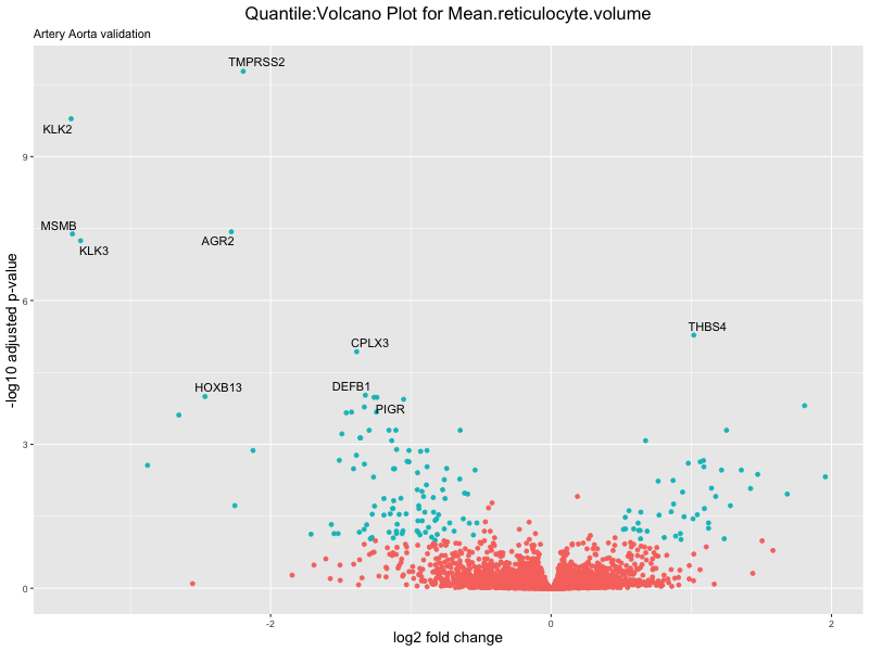
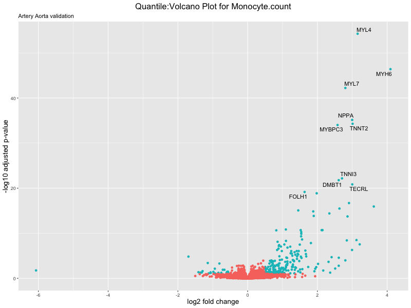
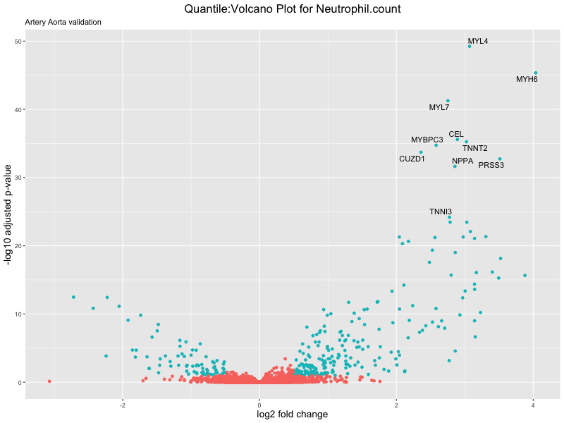
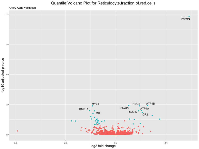
  volcano_plot <- ggplot(res_tableOE, aes(x = log2FoldChange, y = -log10(padj))) +
    geom_point(aes(colour = threshold_OE)) +
    geom_text_repel(aes(label = genelabels)) +
    ggtitle(paste("Quantile:Volcano Plot for", trait), 
            subtitle = "Artery Aorta validation") +
    xlab("log2 fold change") + 
    ylab("-log10 adjusted p-value") +
    theme(legend.position = "none",
          plot.title = element_text(size = rel(1.5), hjust = 0.5),
          axis.title = element_text(size = rel(1.25)))
  
  # Save the volcano plot
  png(paste0("volcano_plot_quantile_", trait, "_artery_validation.png"), width = 800, height = 600)
  print(volcano_plot)
  dev.off()
}

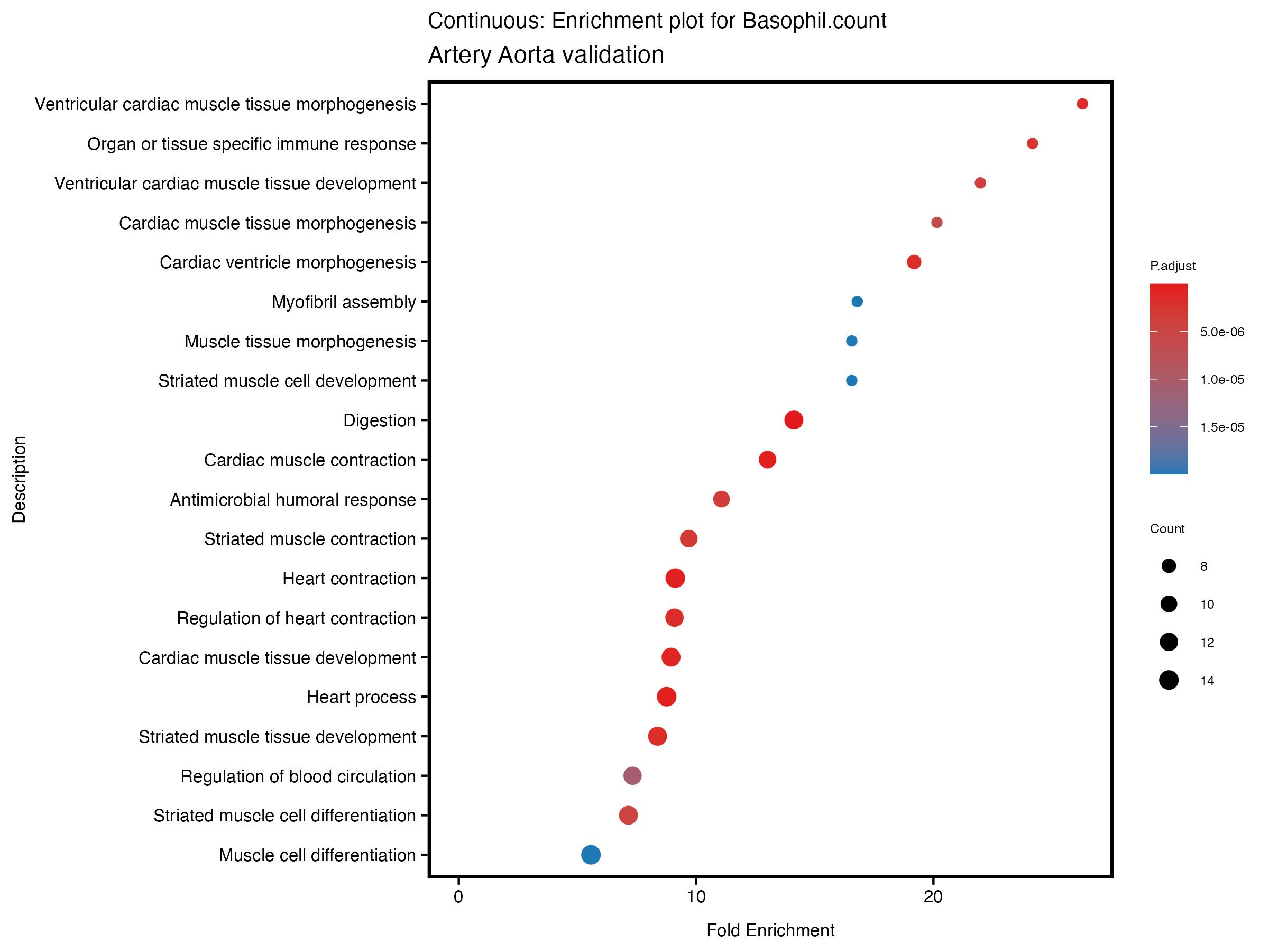
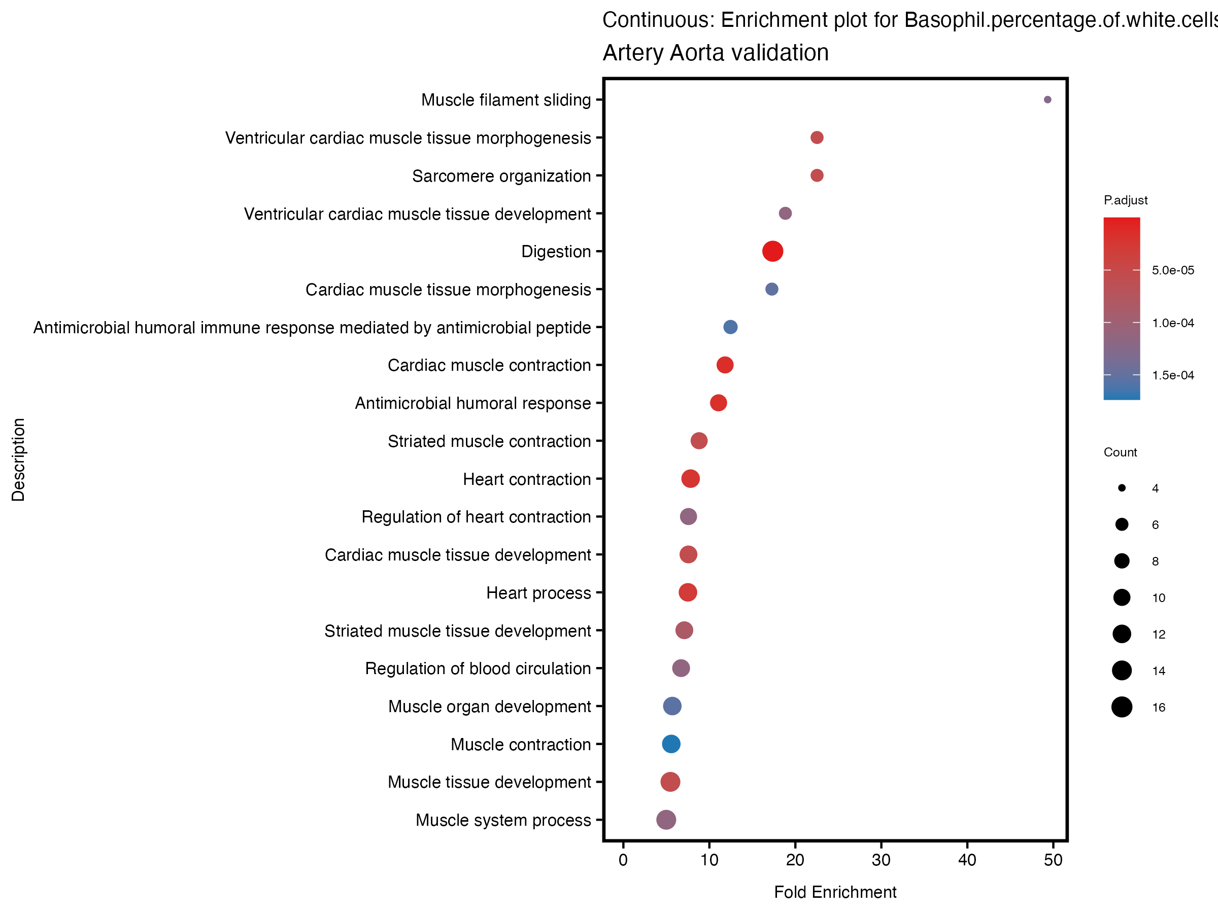
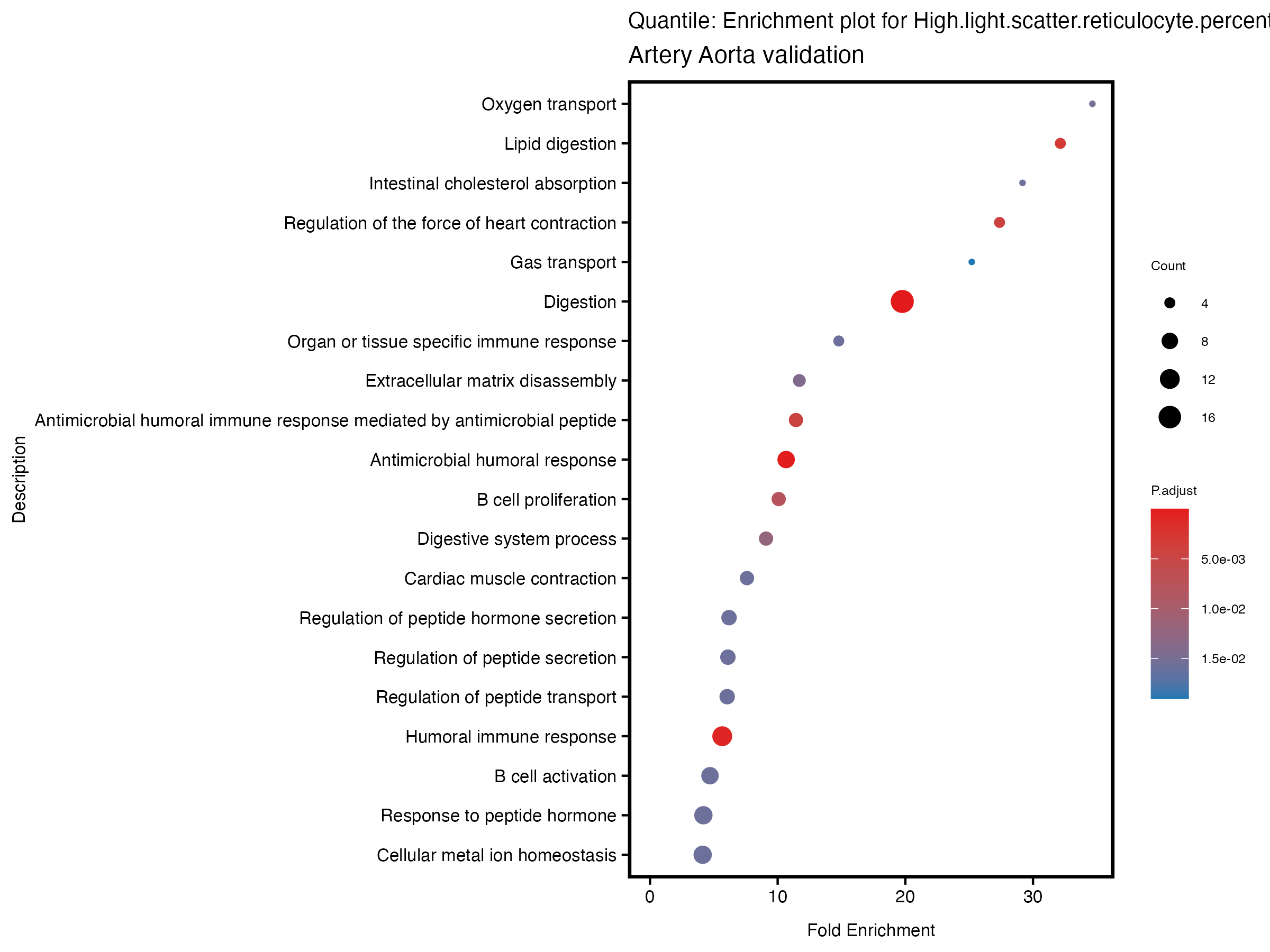
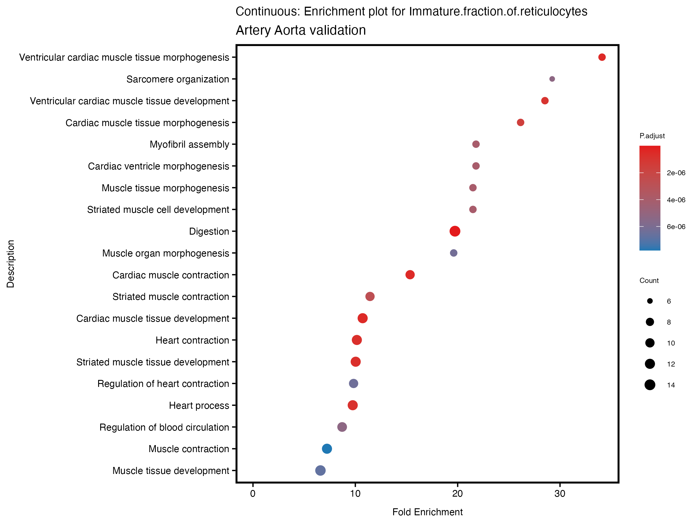
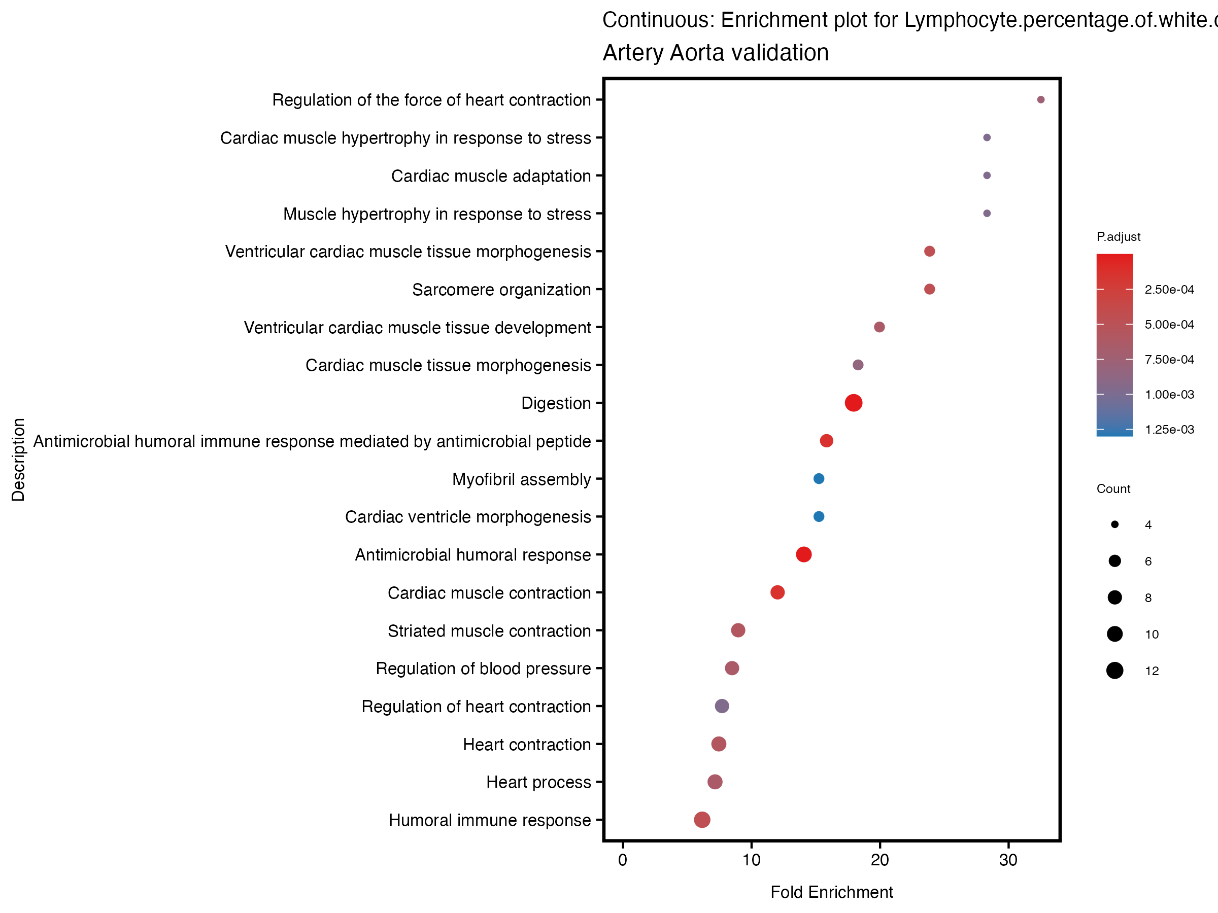
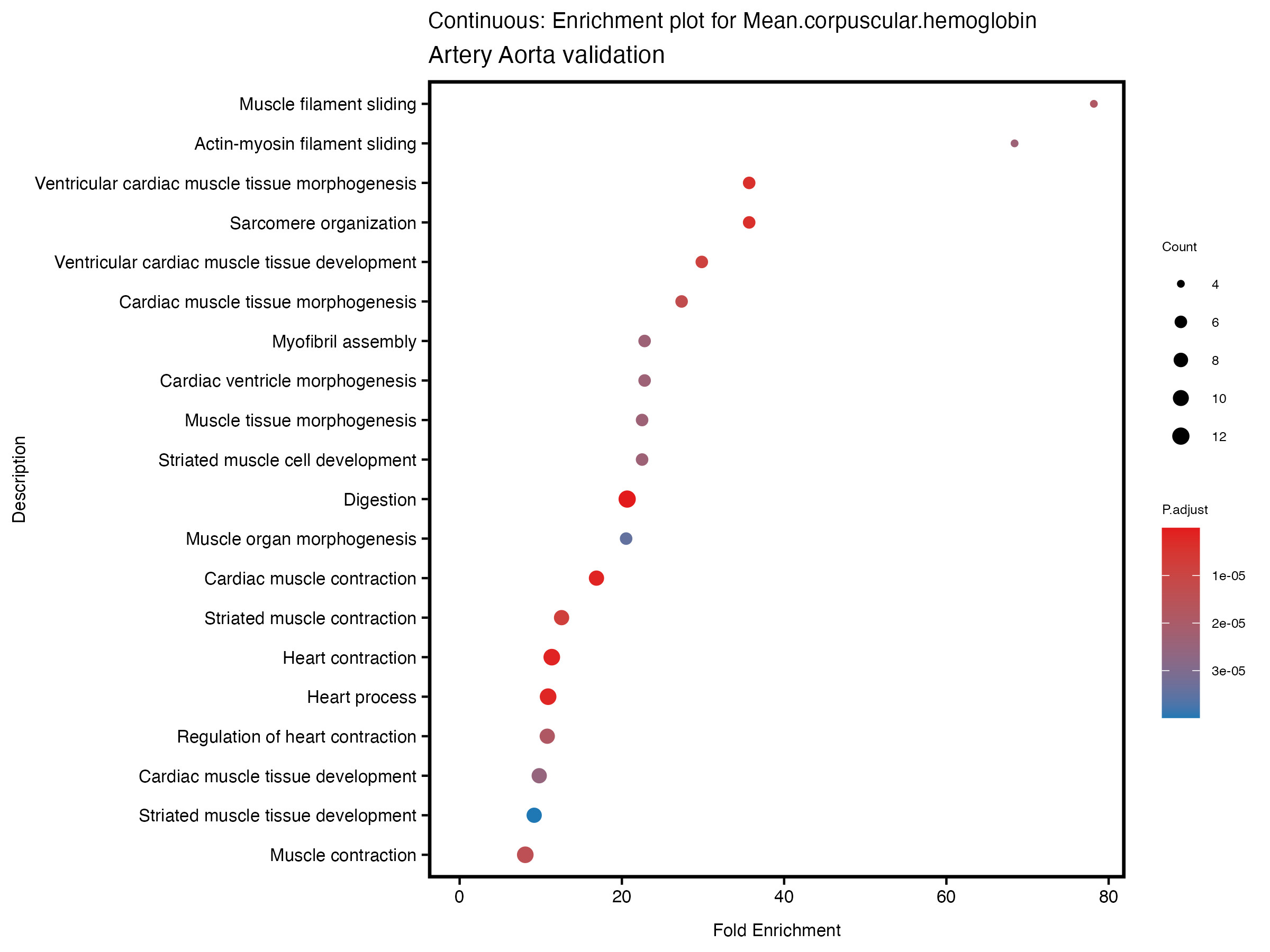
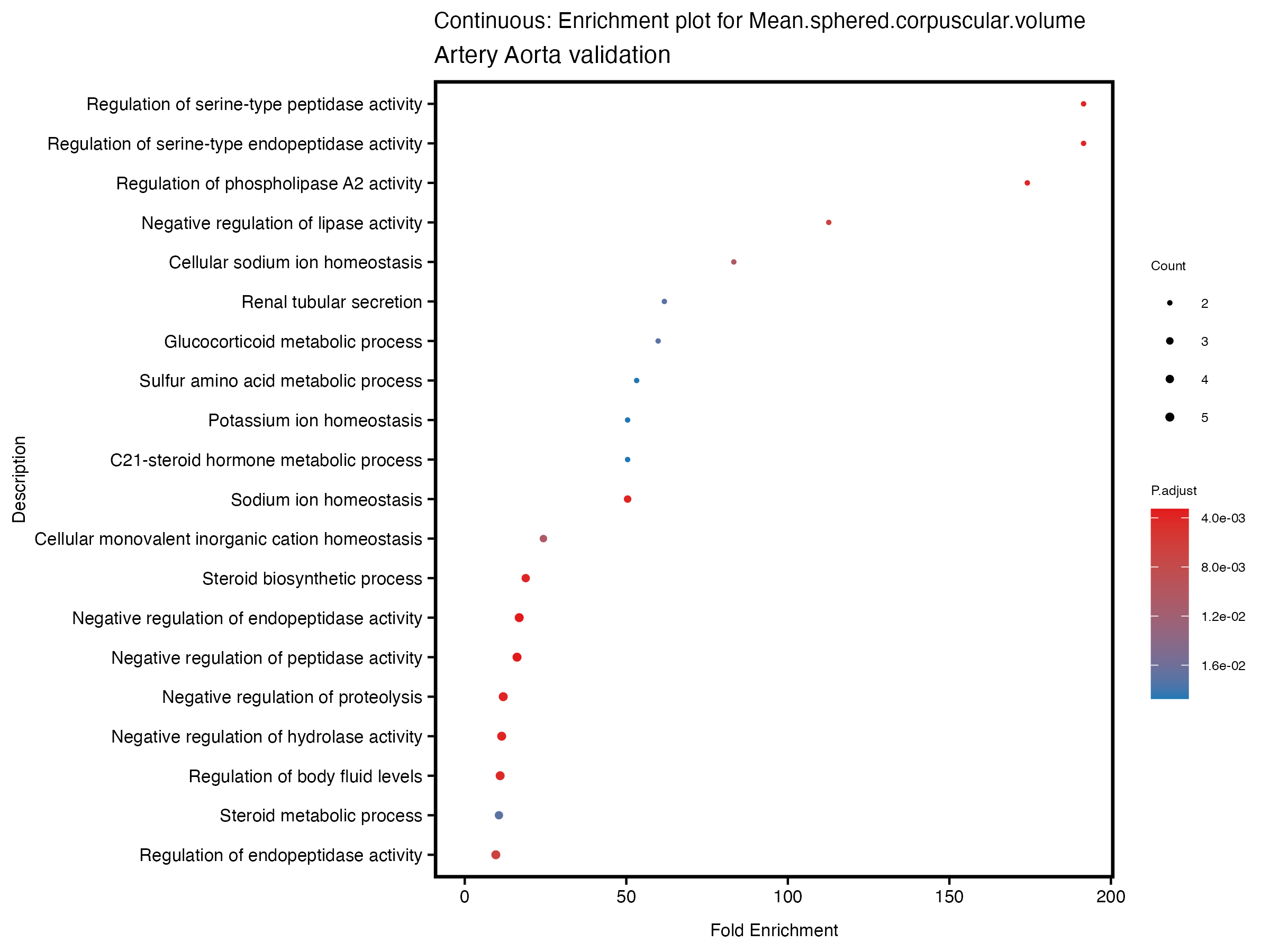
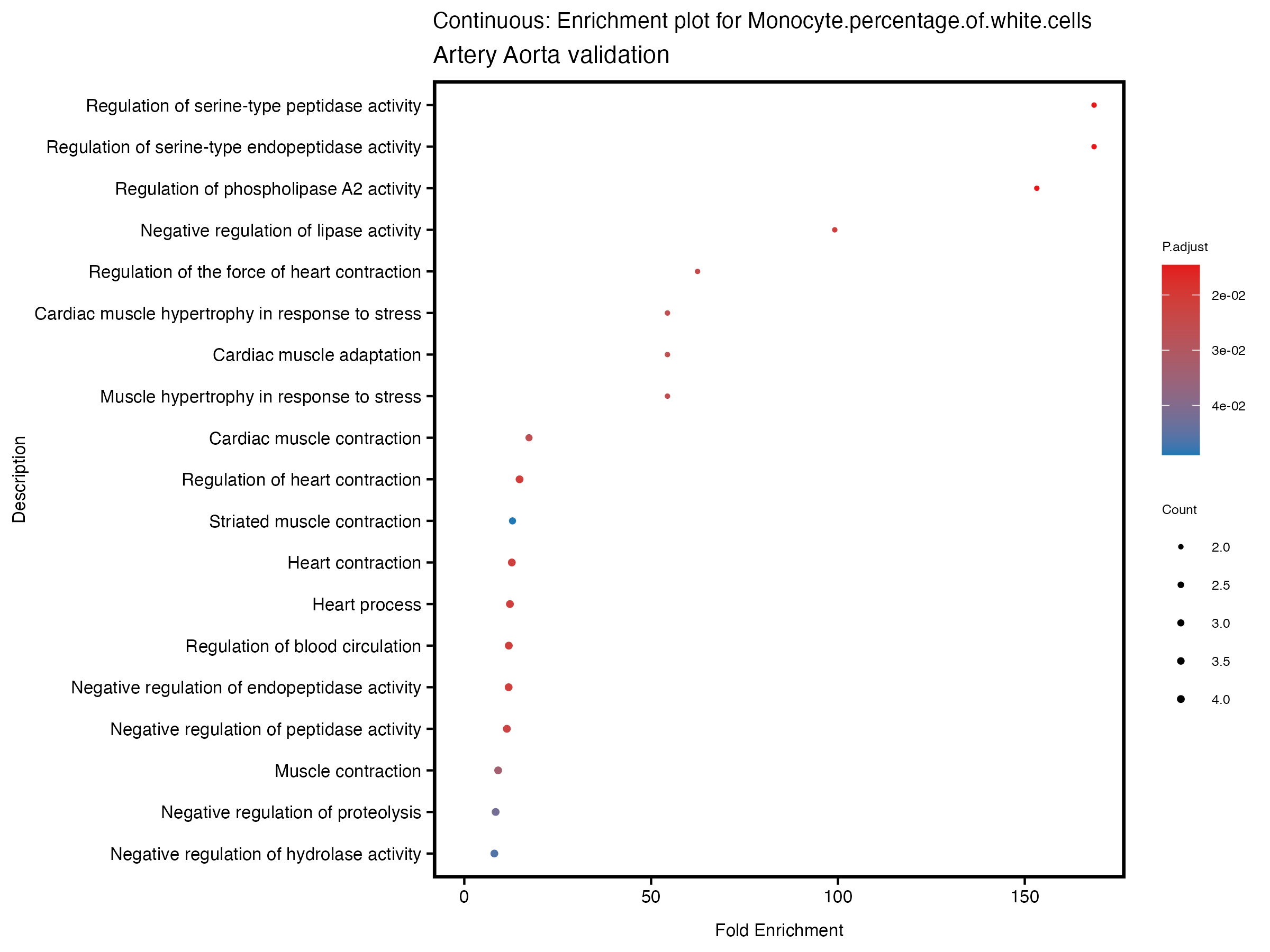
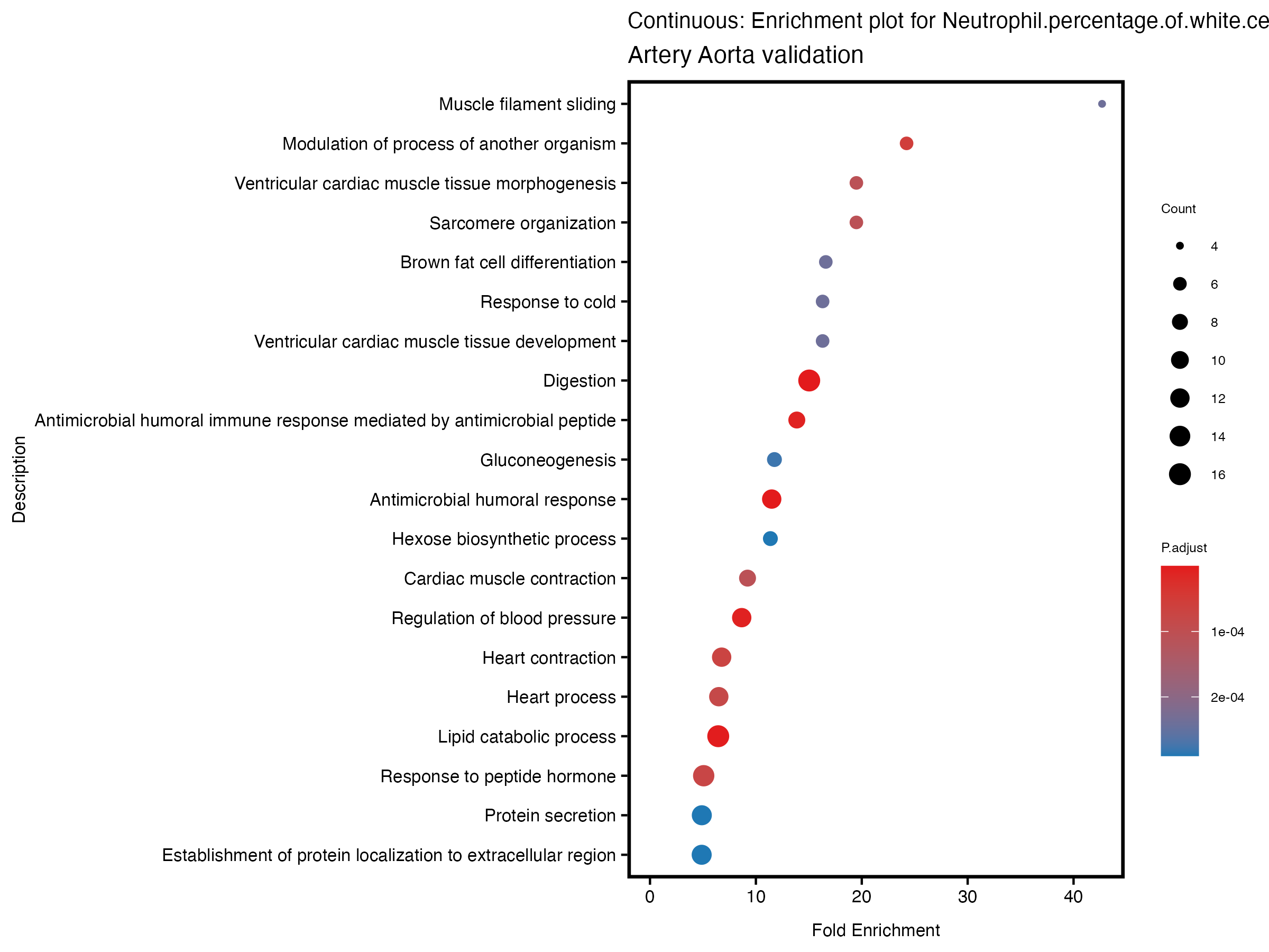
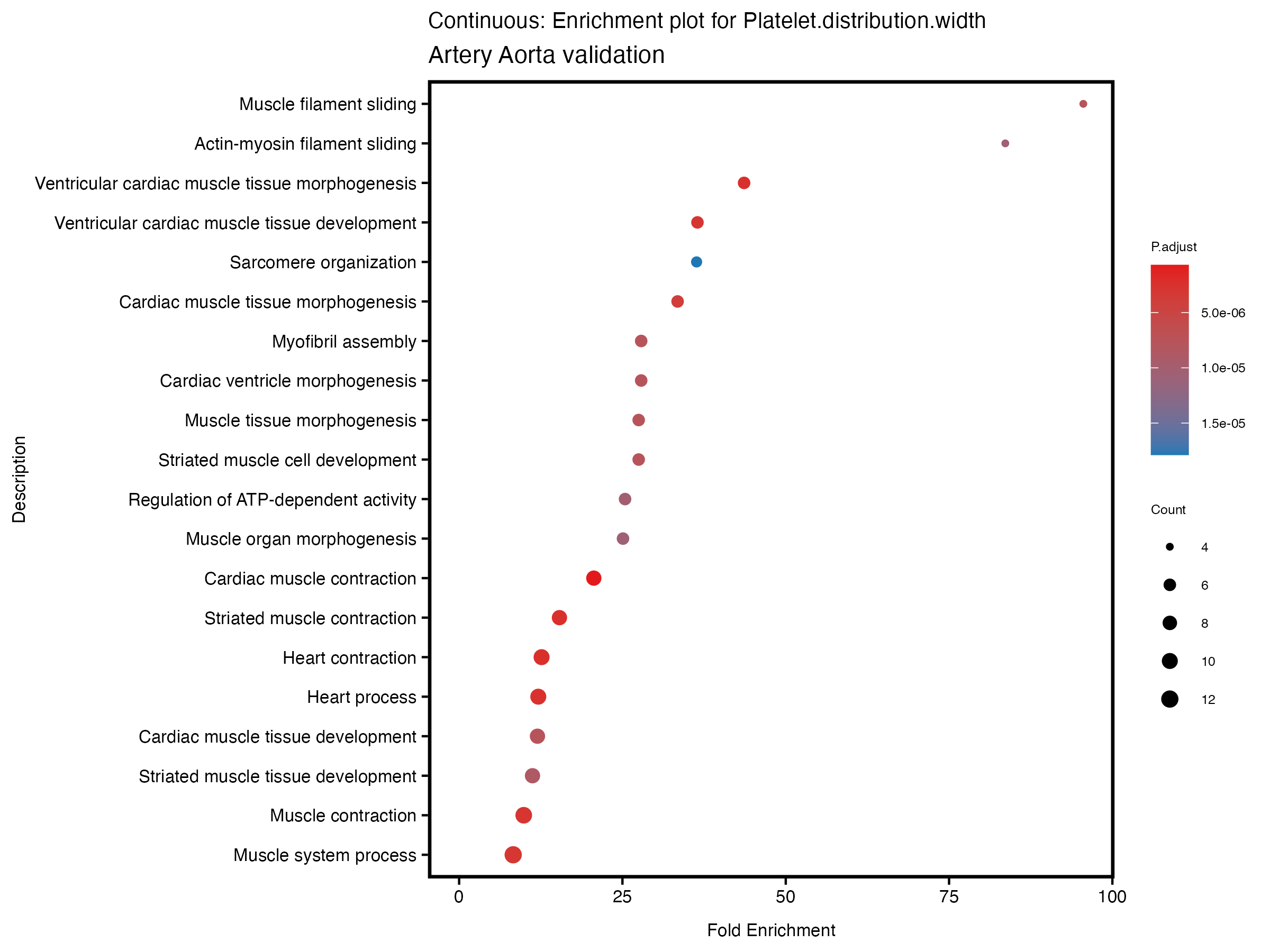
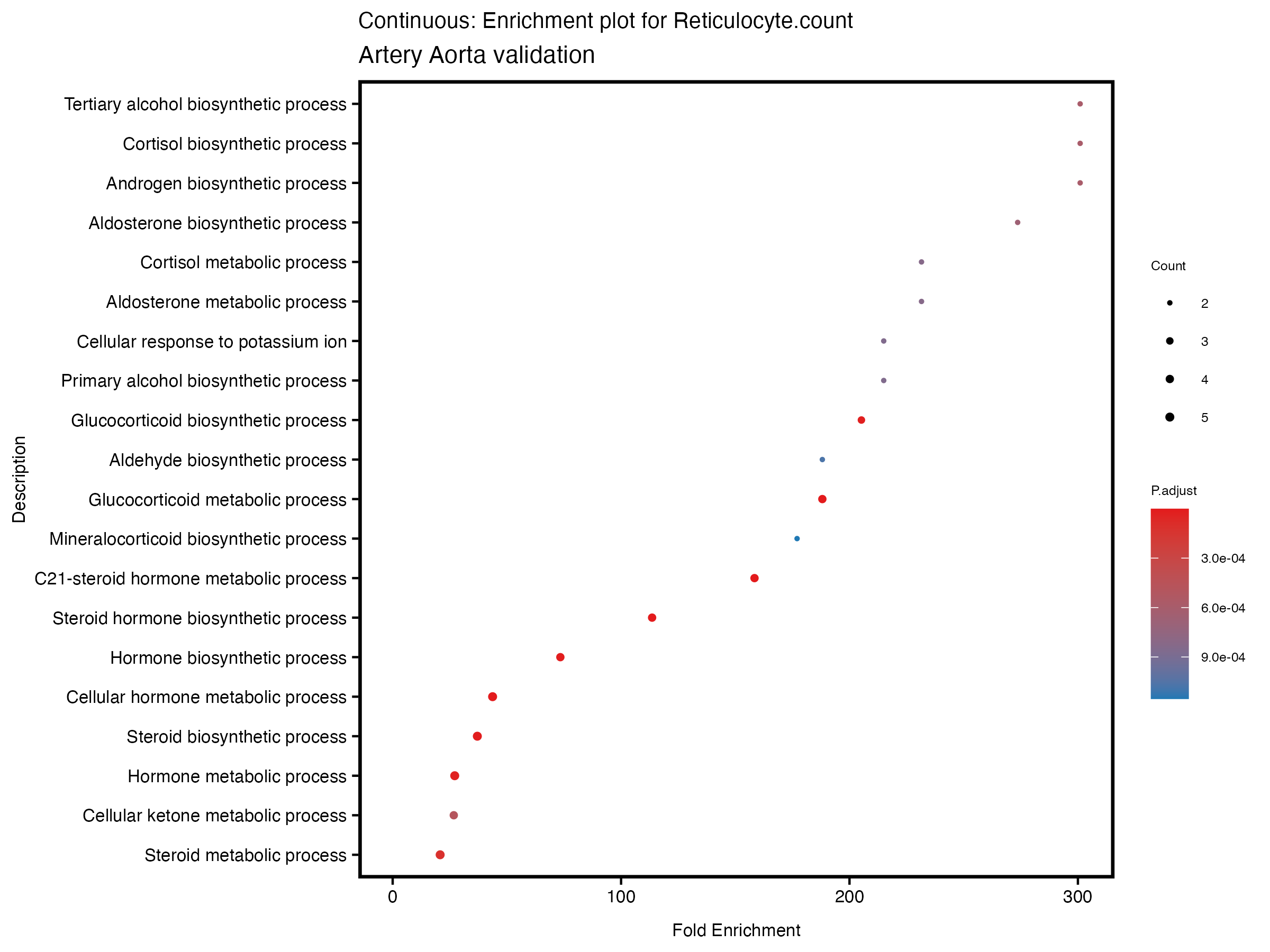
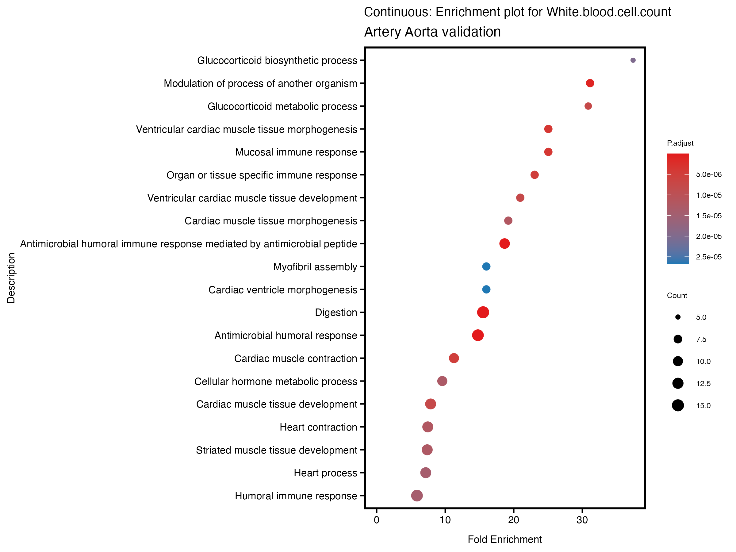
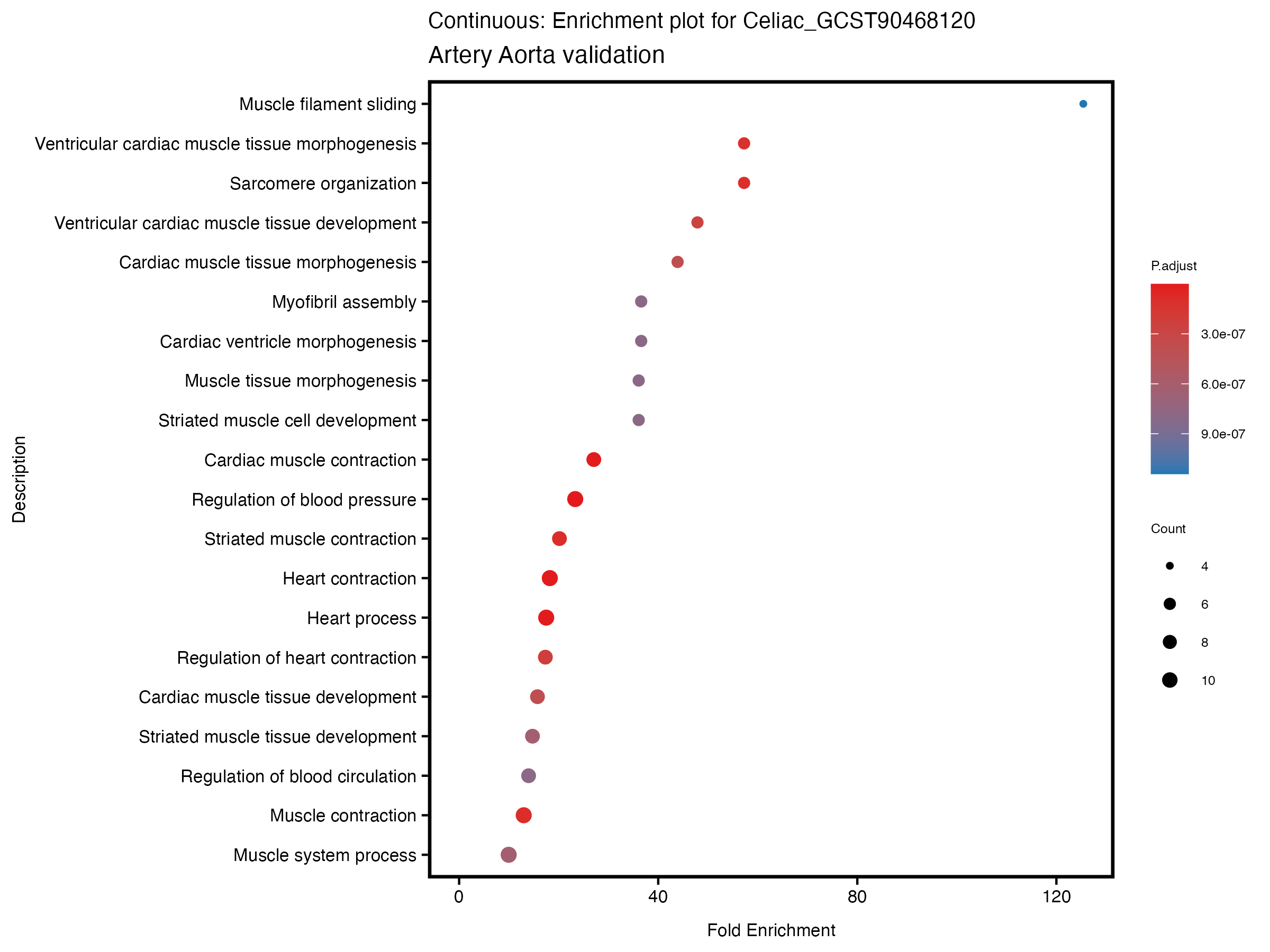
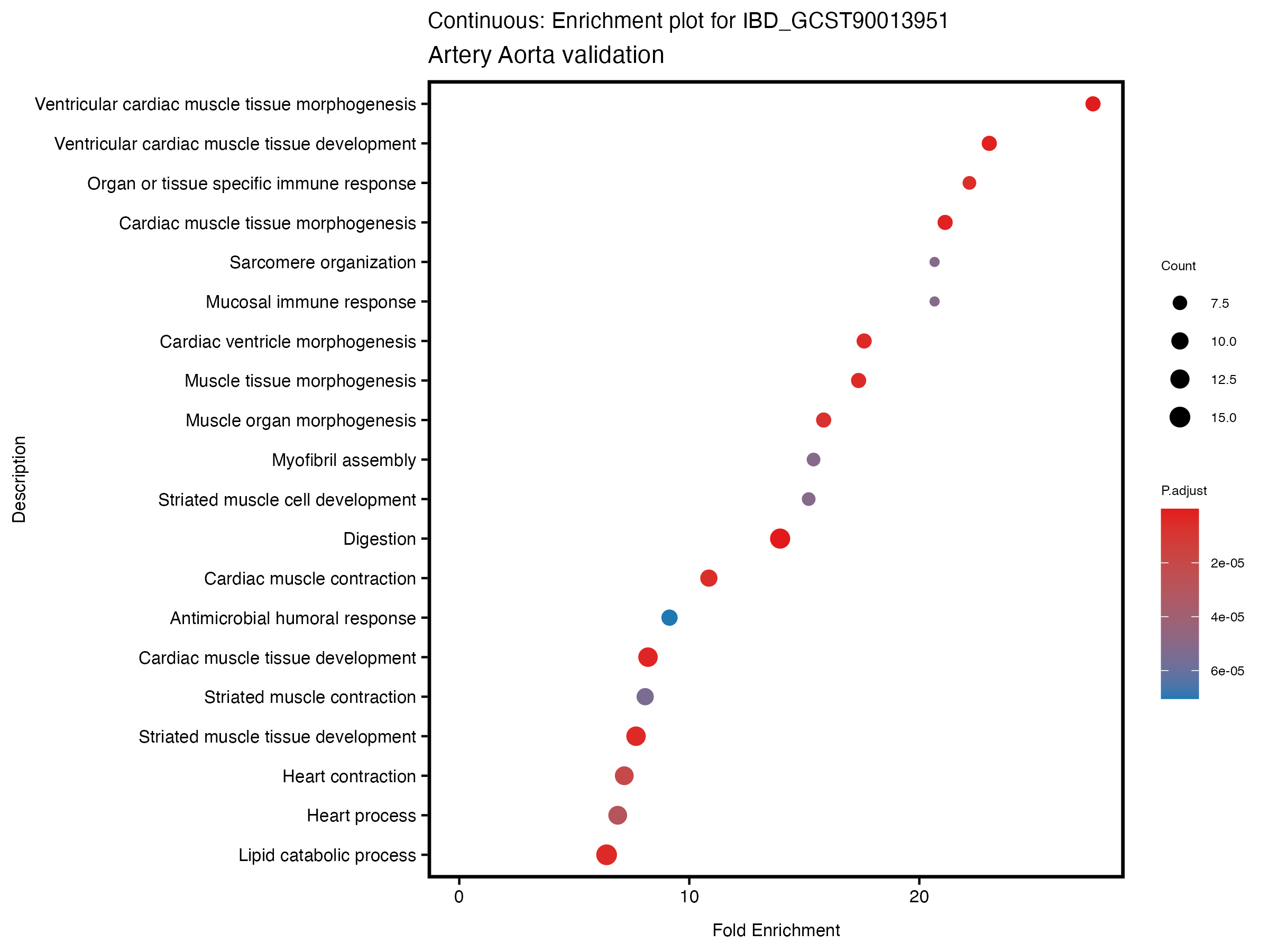
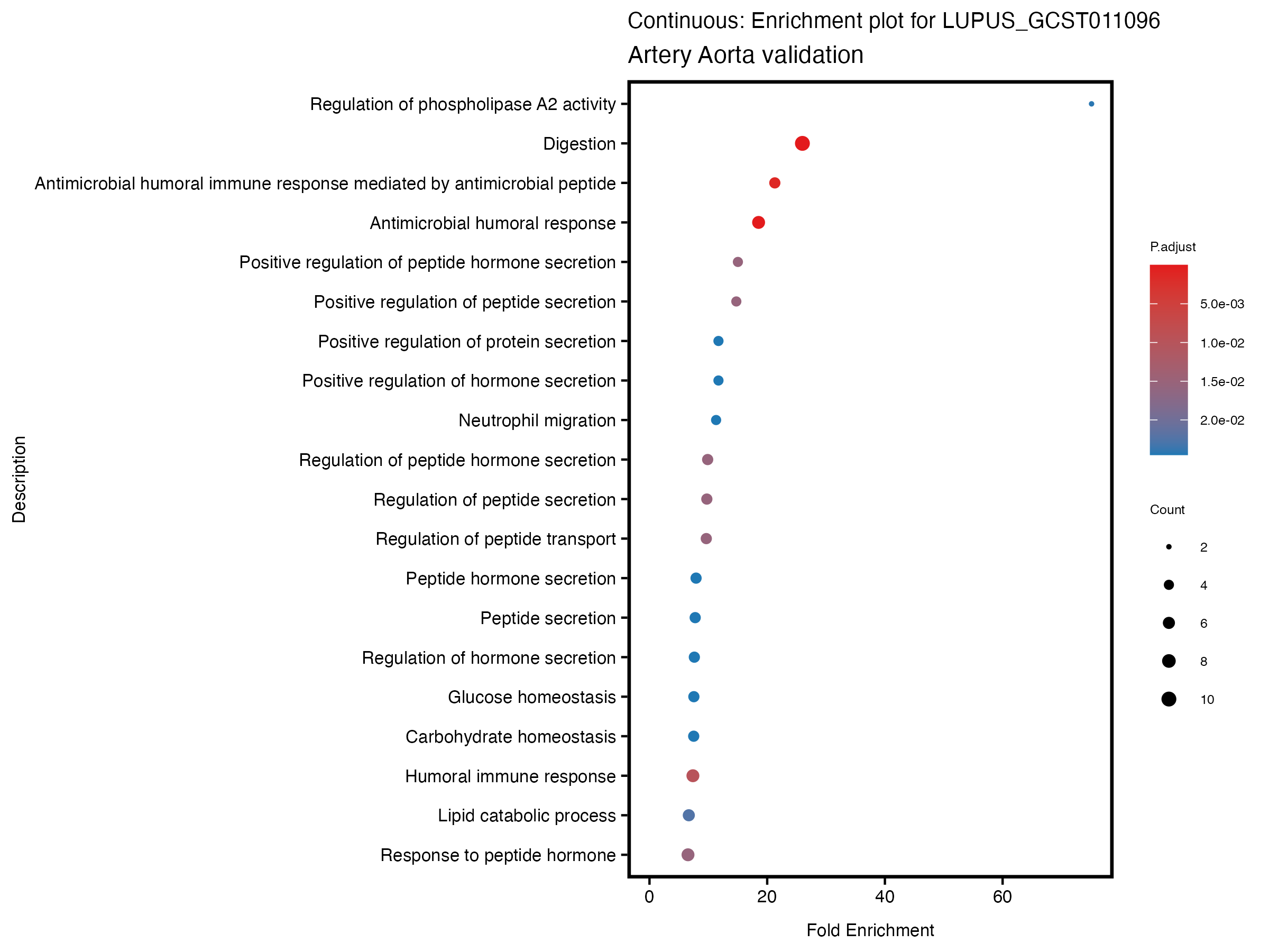
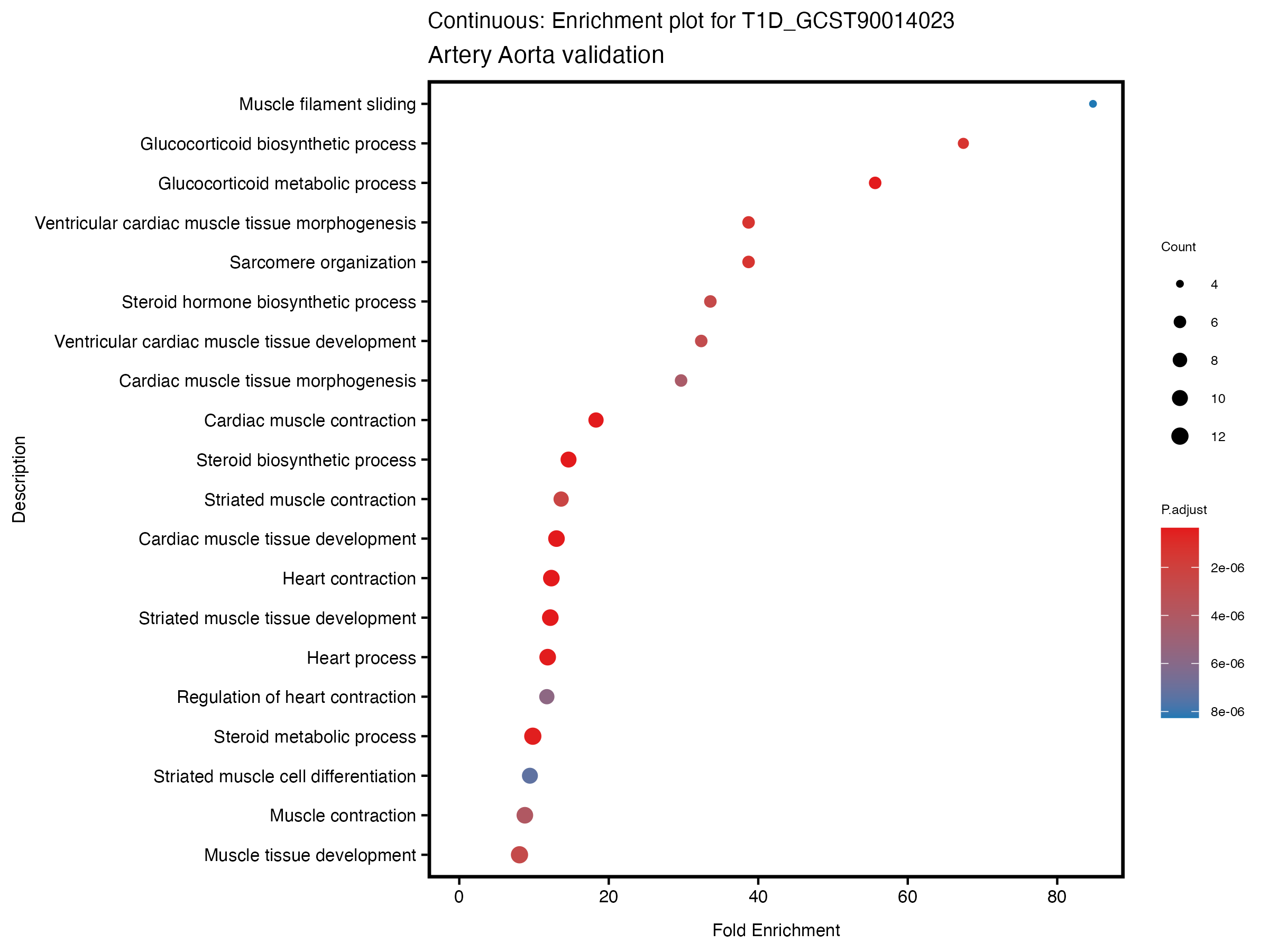
Gene enrichment Analysis

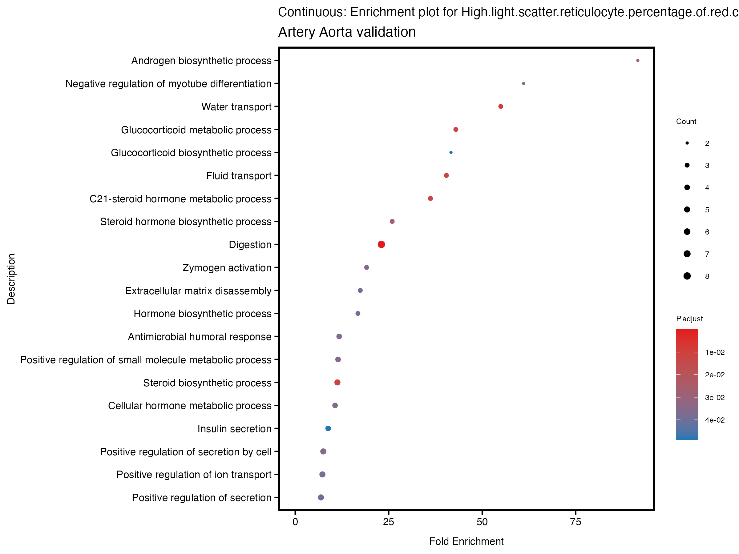
BgRatio: Number of all genes in specific GO term / Number of universal genes

GeneRatio: Number of genes enriched in specific term / Number of input genes

FoldEnrichment: GeneRatio / BgRatio

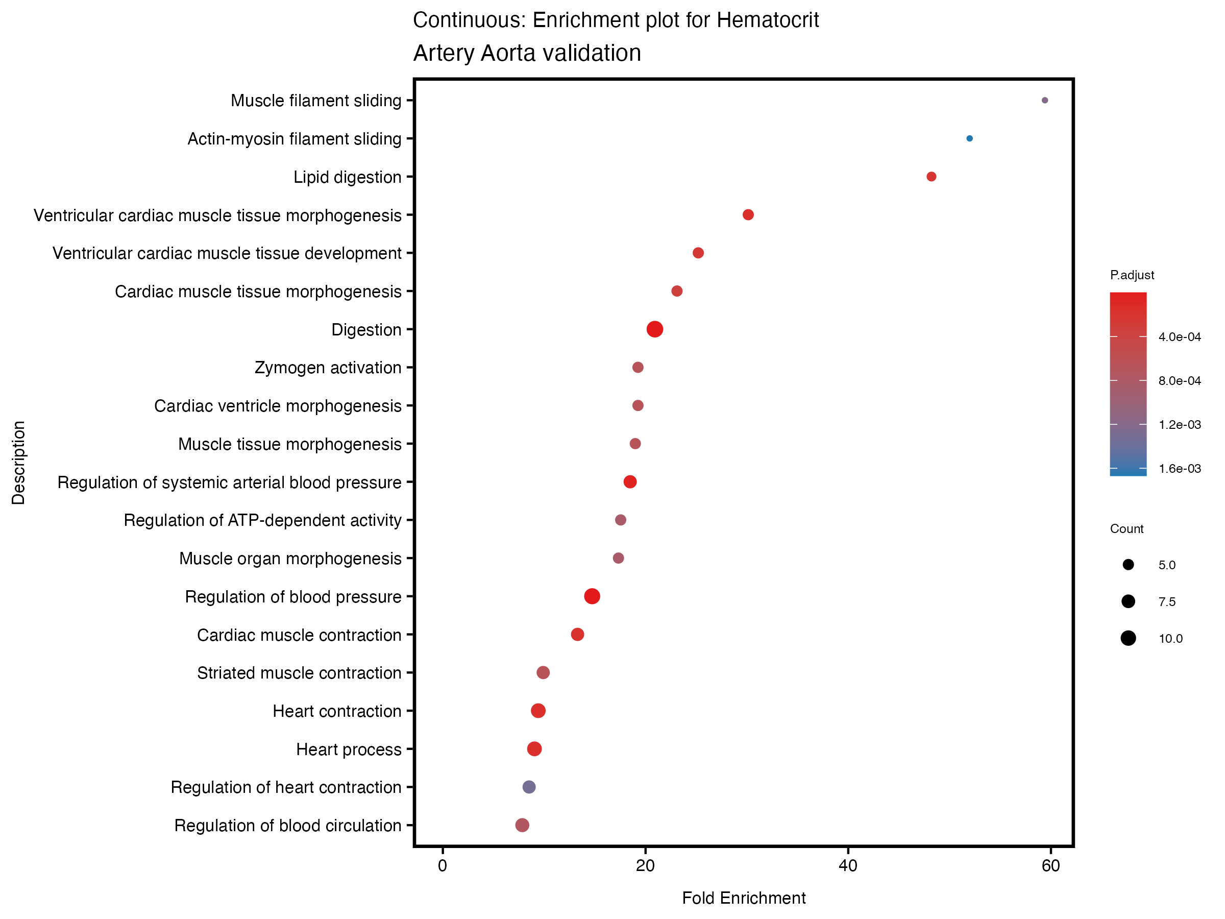
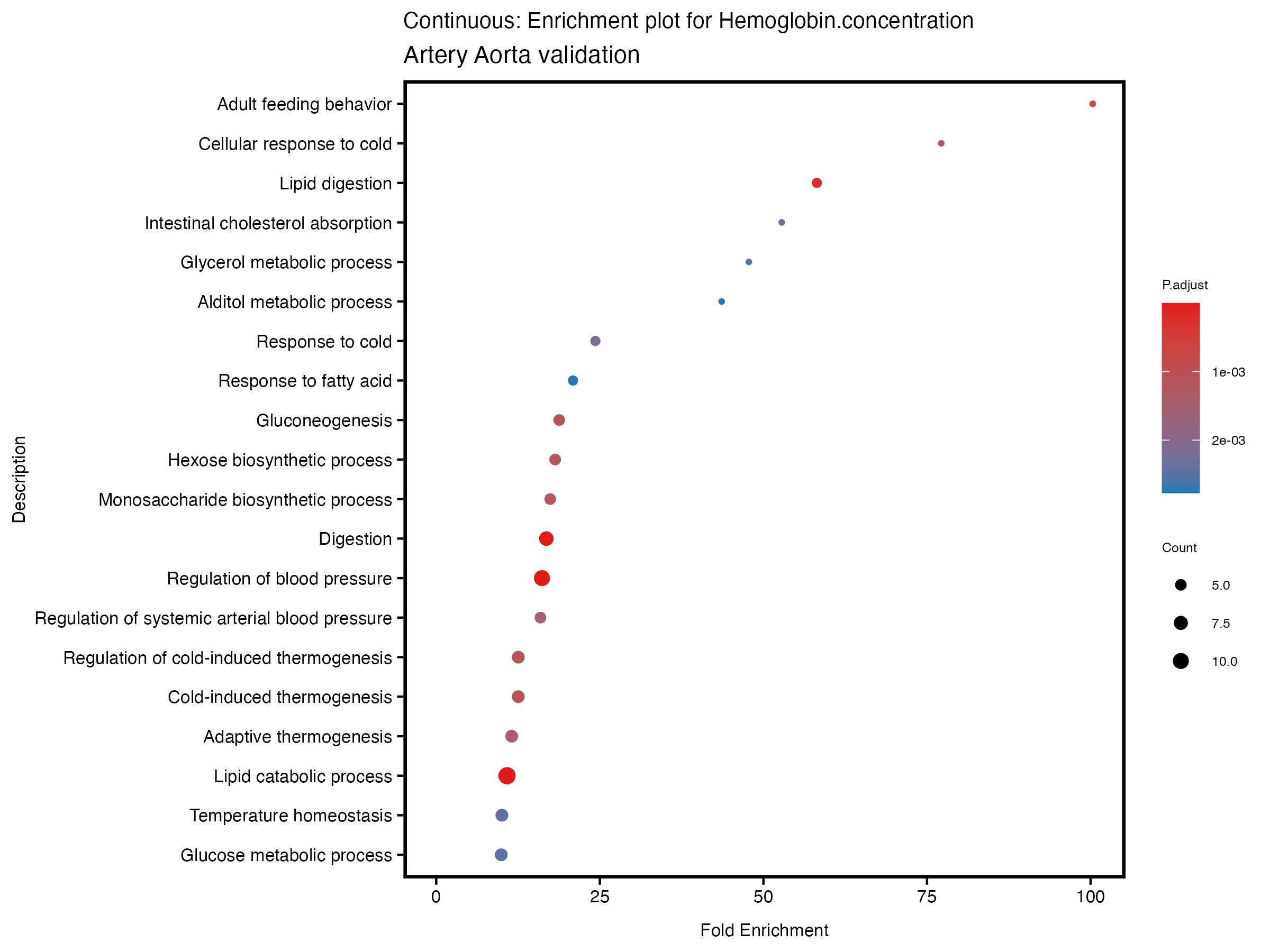
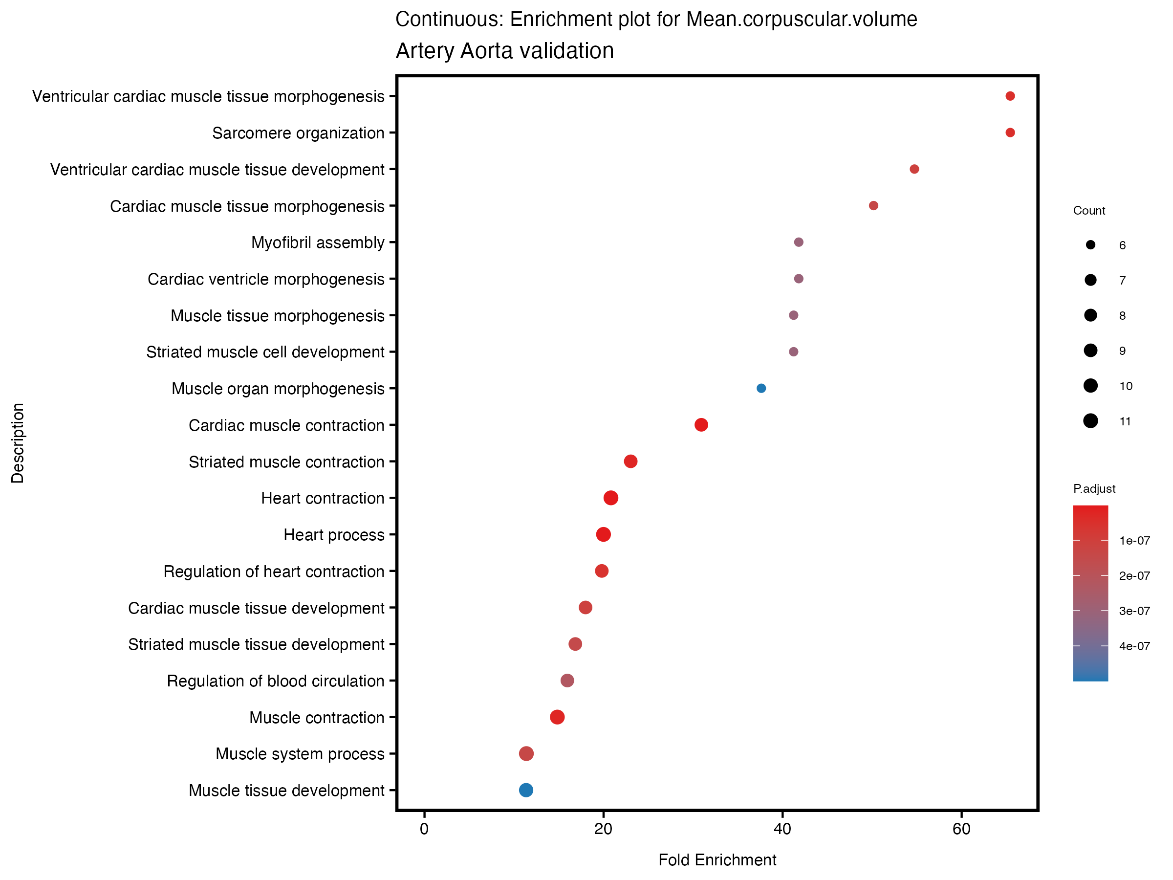
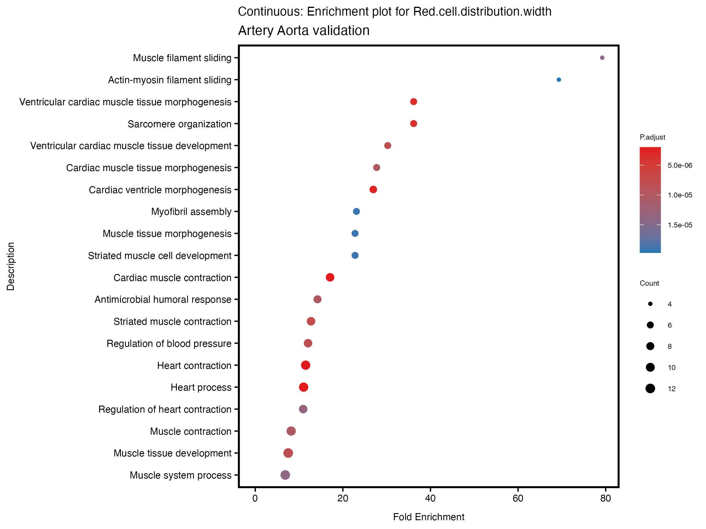
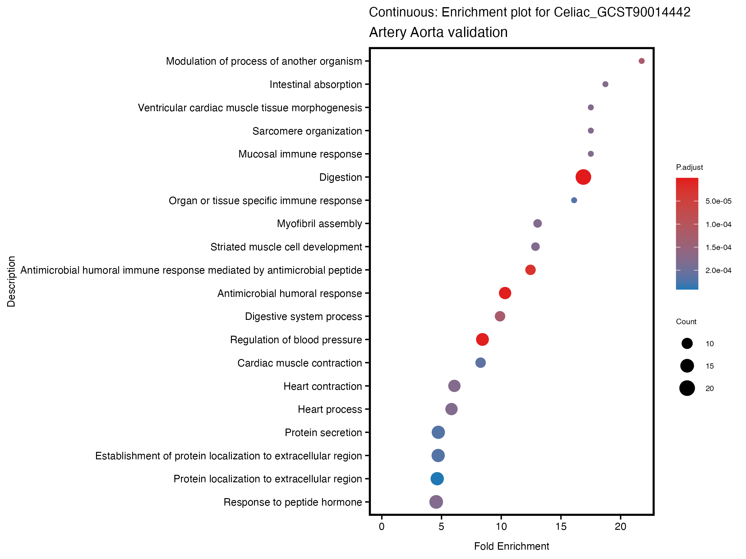
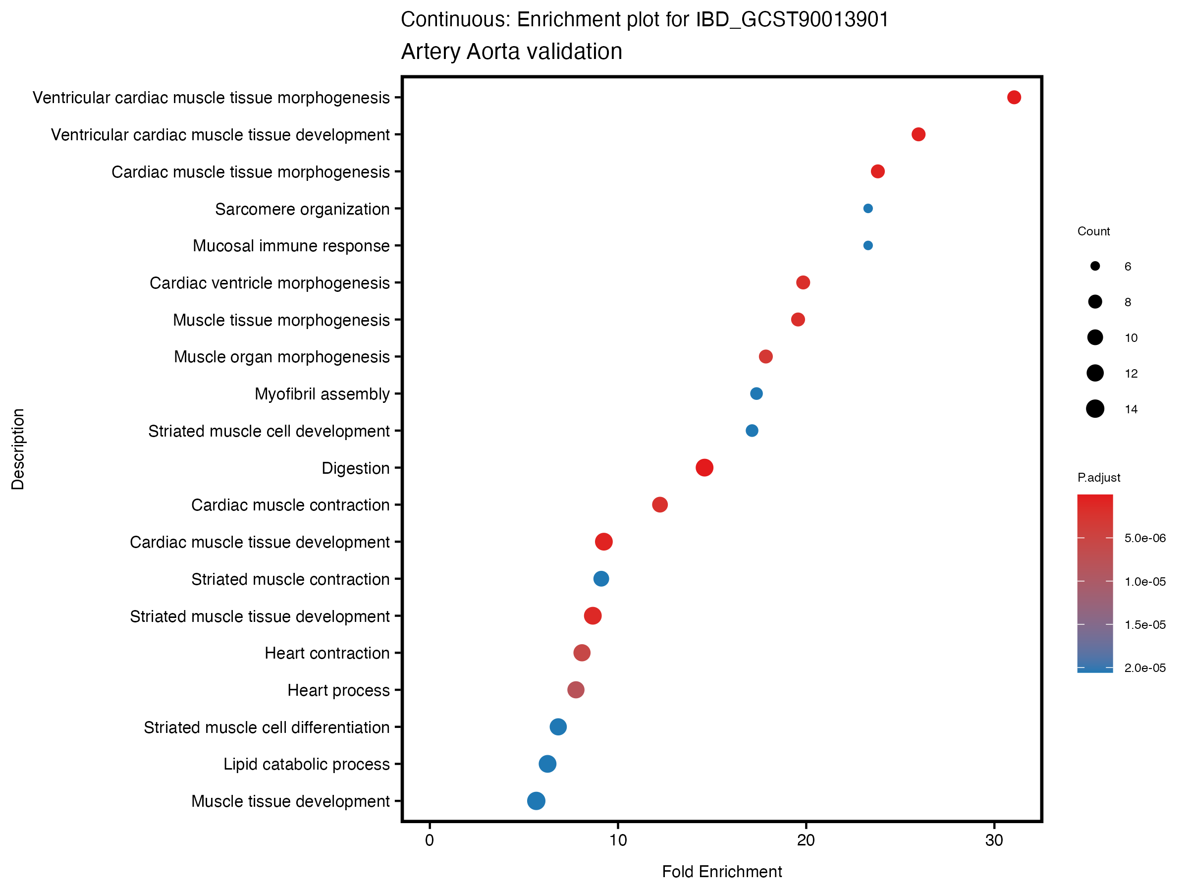
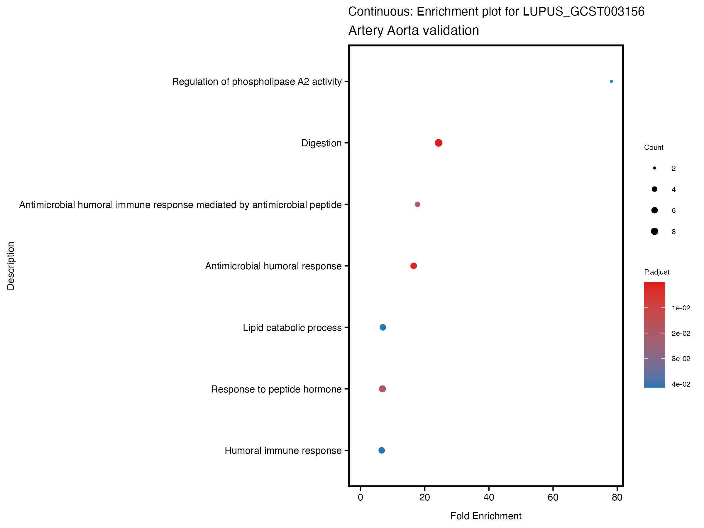
# continous
dir_path <- "analysis/continuous_artery"
files <- list.files(dir_path, pattern = "differential_expression_.*_results_artery_validation.csv", full.names = TRUE)

for (file in files) {
  trait <- gsub("differential_expression_(.*)_results_artery_validation.csv", "\\1", basename(file))
  trait
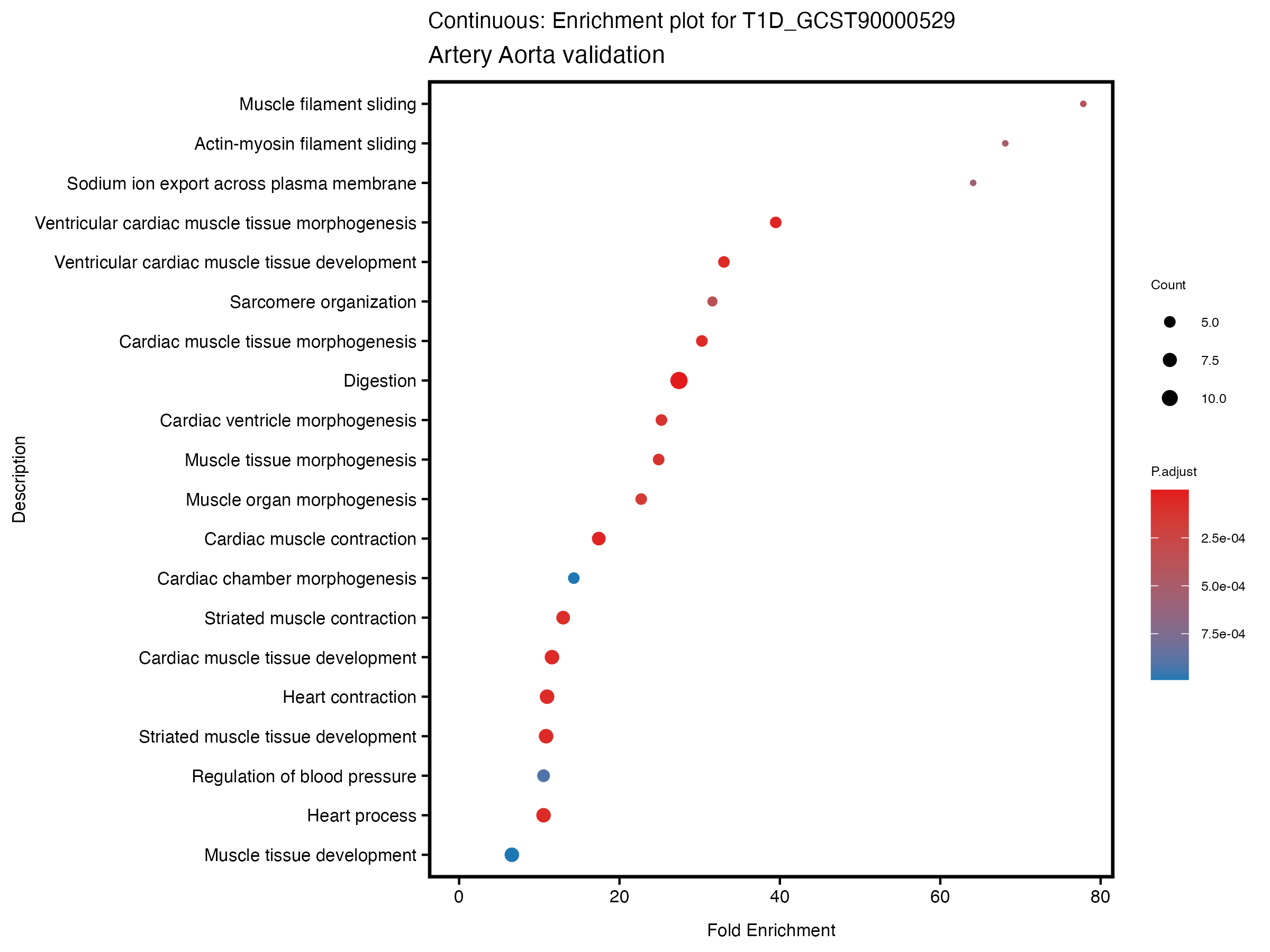
  res_tableOE <- read.csv(file, header = T, row.names = 1)
  
  deGenes <- res_tableOE[res_tableOE$padj < 0.1 & 
                           abs(res_tableOE$log2FoldChange) >= 0.5, ]
  deGenes$gene_id <- gsub("\\.\\d+$", "", rownames(deGenes))
  
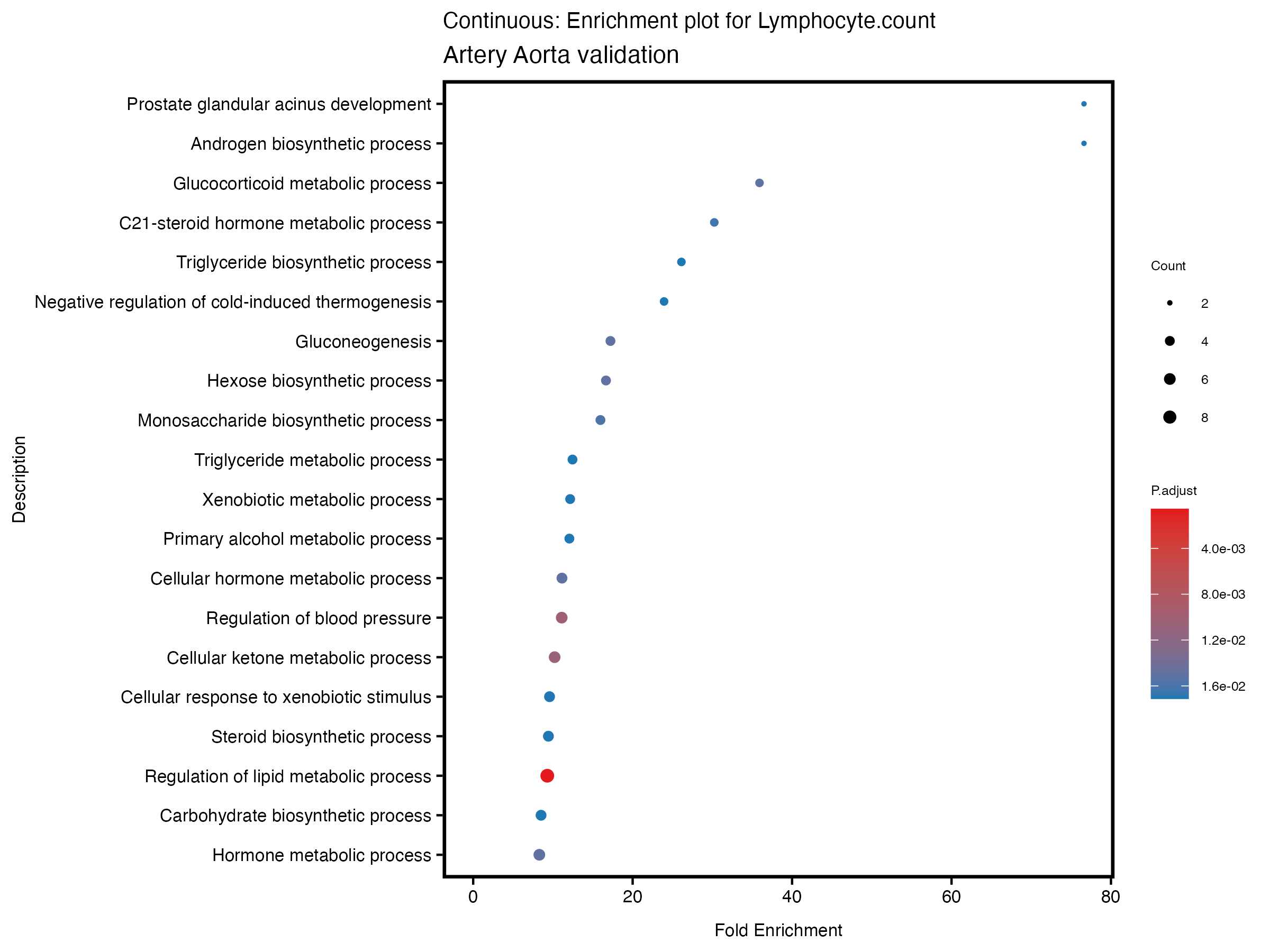
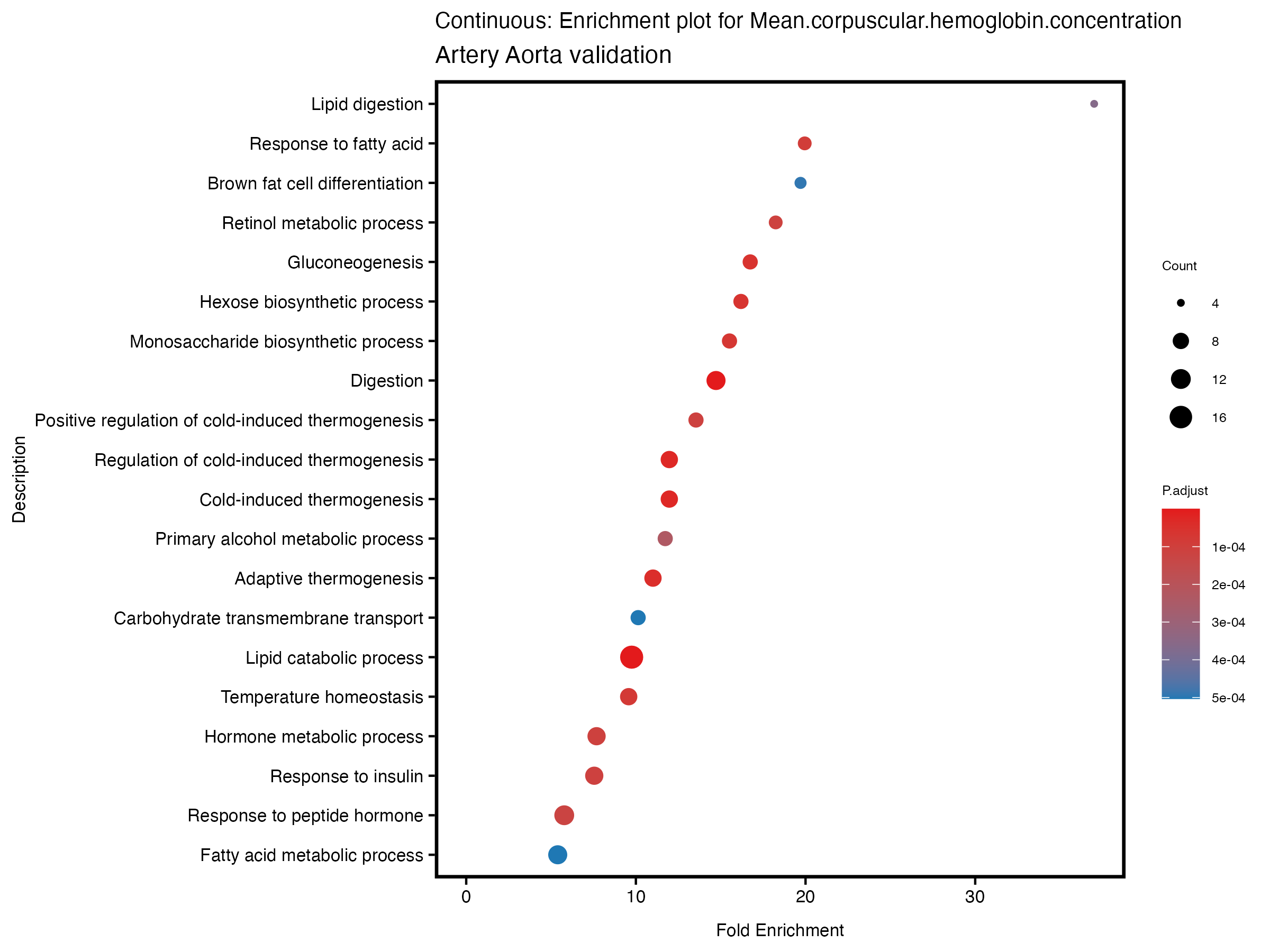
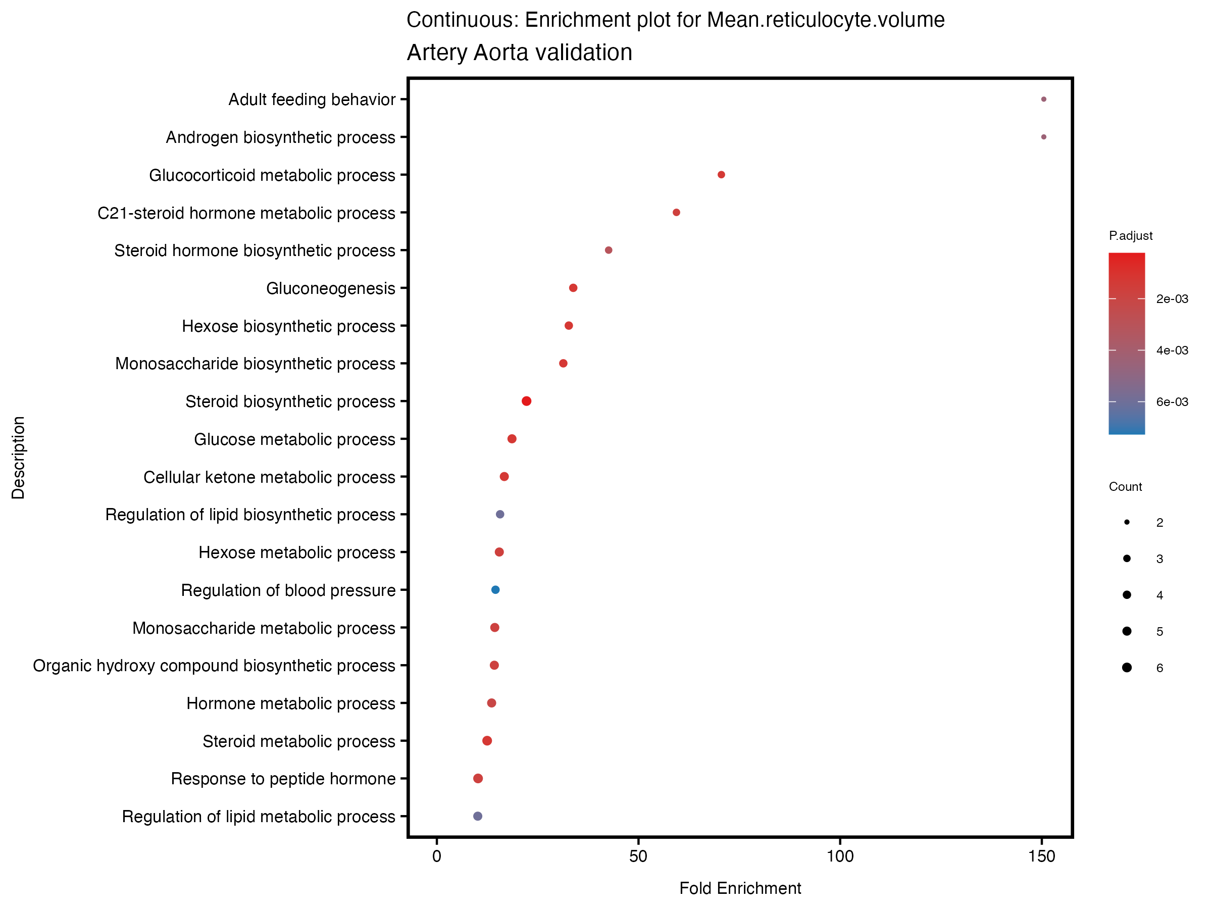
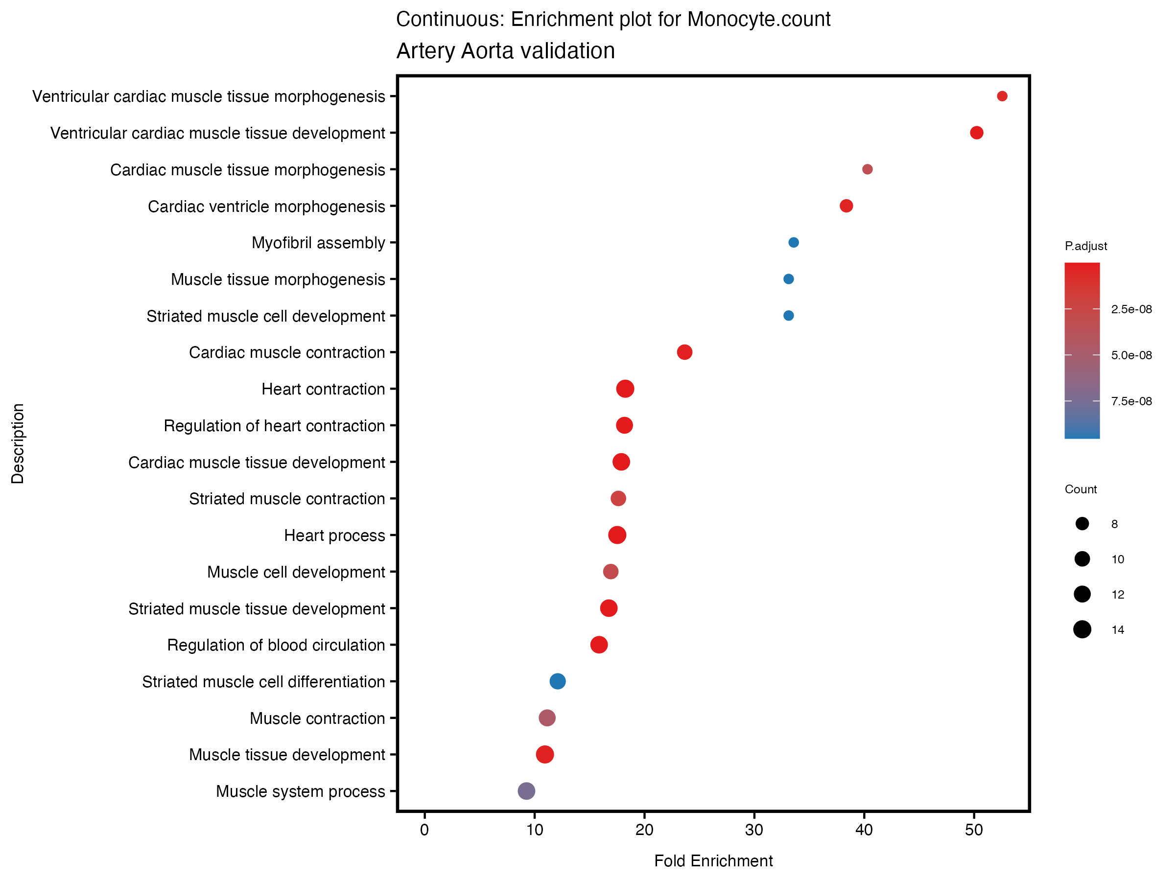
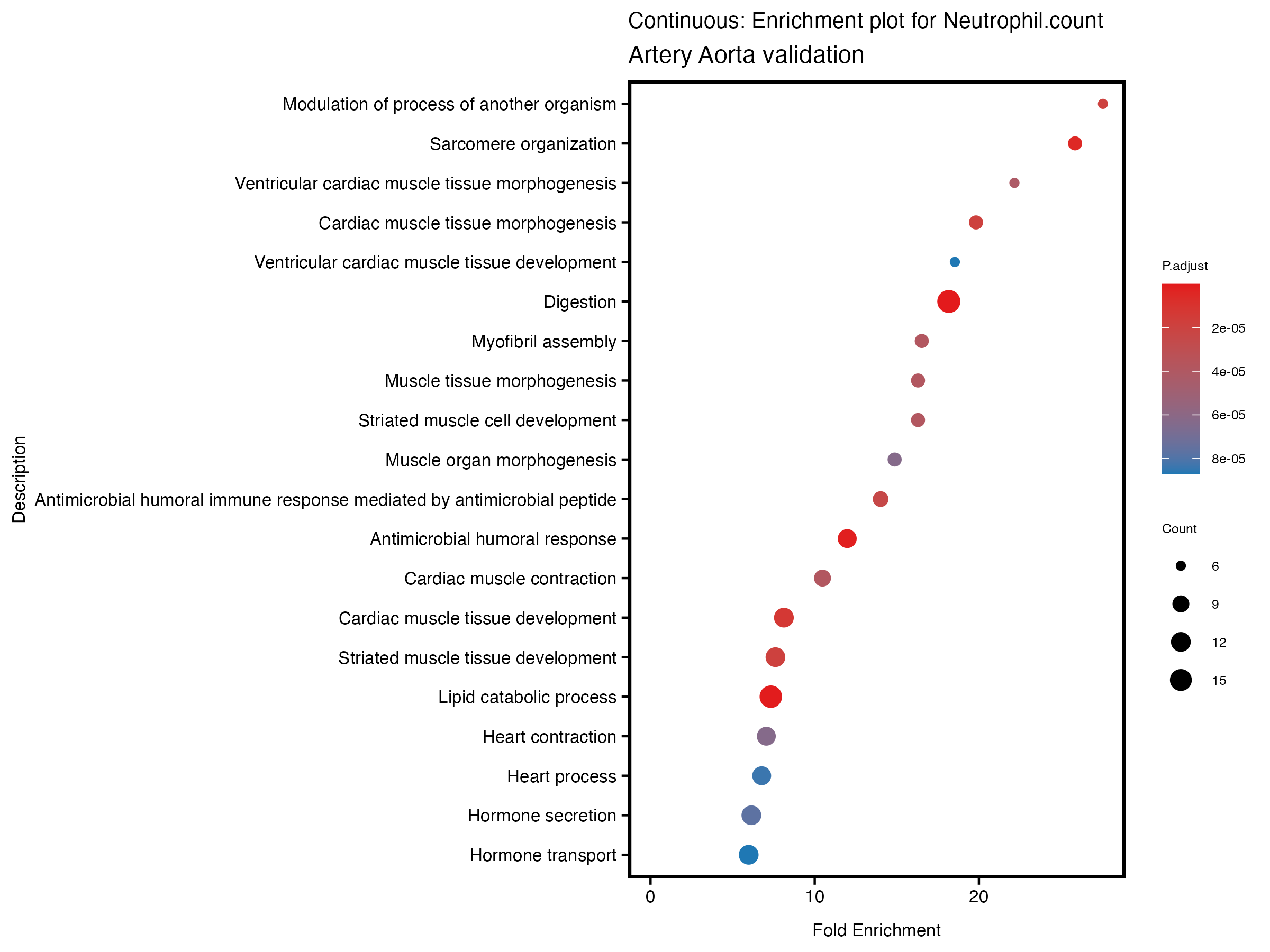
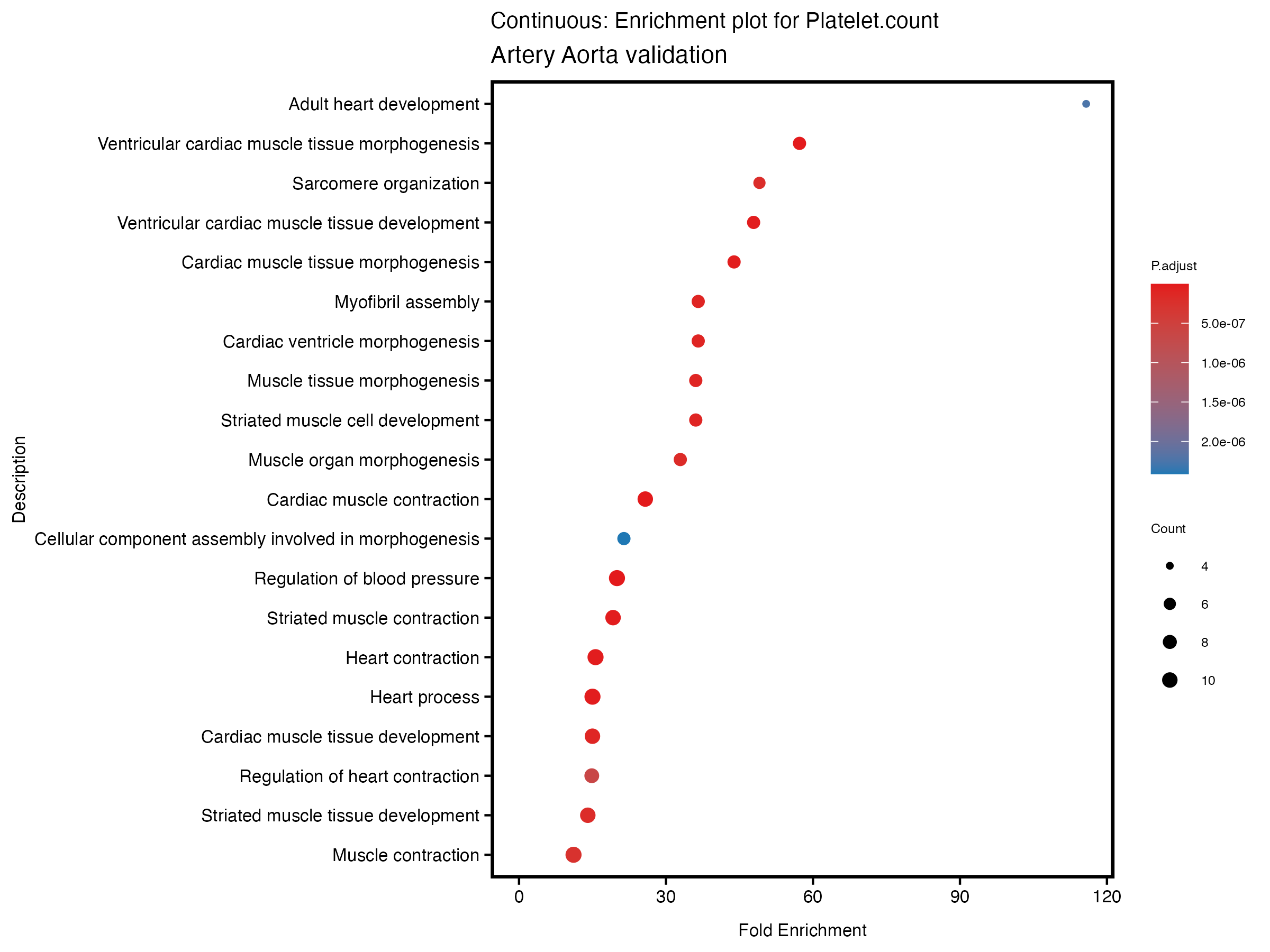
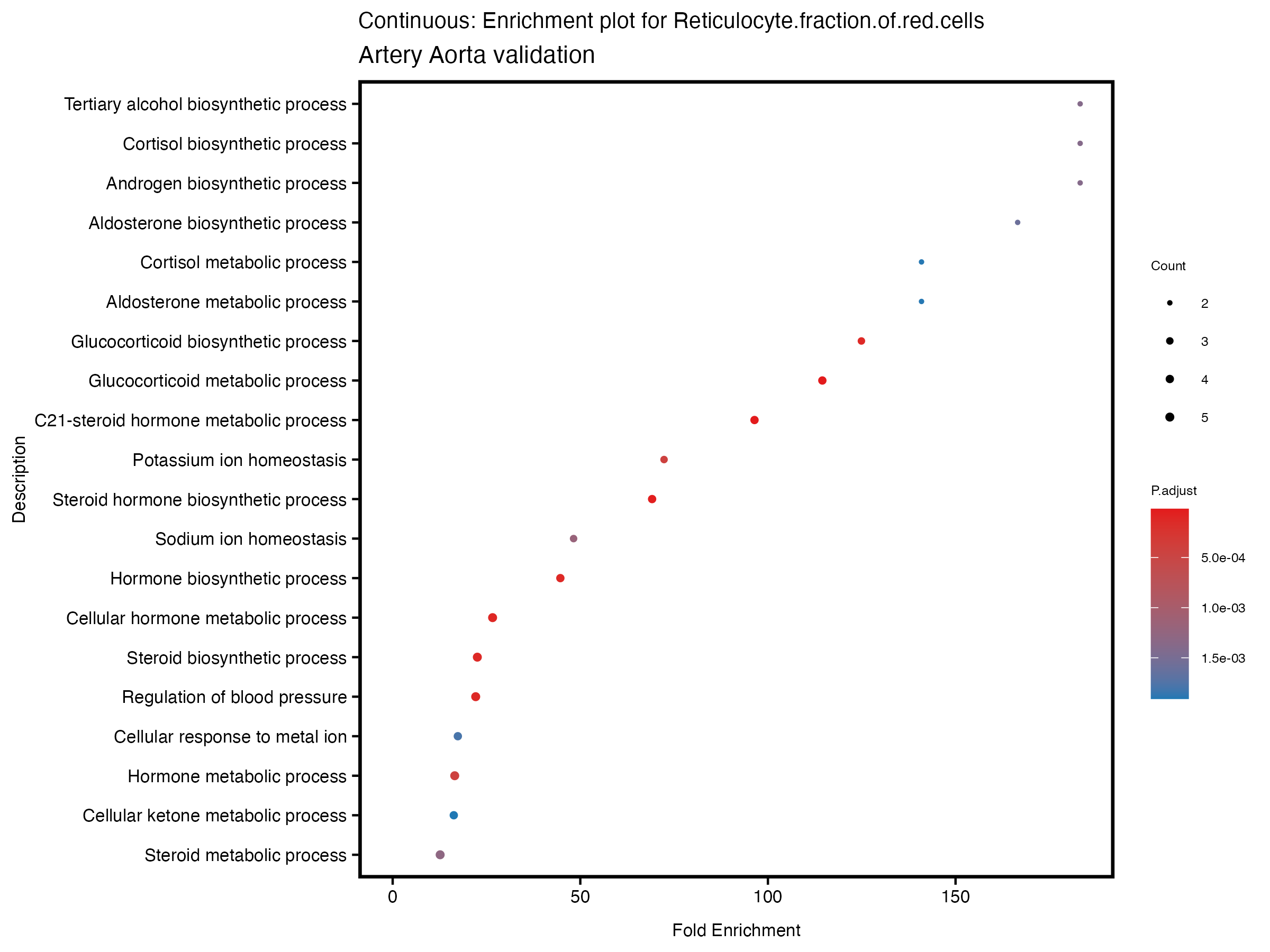
  gse <- enrichGO(gene = deGenes$gene_id, ont = "BP", 
                OrgDb ="org.Hs.eg.db", keyType = "ENSEMBL")
  
  write.csv(as.data.frame(gse), file = paste0("GO_enrichment_", trait, "_results_artery_validation.csv"))
  
  gse <- as.data.frame(gse)
  gse$GeneRatio_num <- as.numeric(sapply(strsplit(gse$GeneRatio, "/"), 
                                         function(x) x[1])) /
                     as.numeric(sapply(strsplit(gse$GeneRatio, "/"), function(x) x[2]))

  gse$BgRatio_num <- as.numeric(sapply(strsplit(gse$BgRatio, "/"), function(x) x[1])) / 
                     as.numeric(sapply(strsplit(gse$BgRatio, "/"), function(x) x[2]))
  
  gse <- cbind(gse, FoldEnrich = gse$GeneRatio_num/gse$BgRatio_num)
  
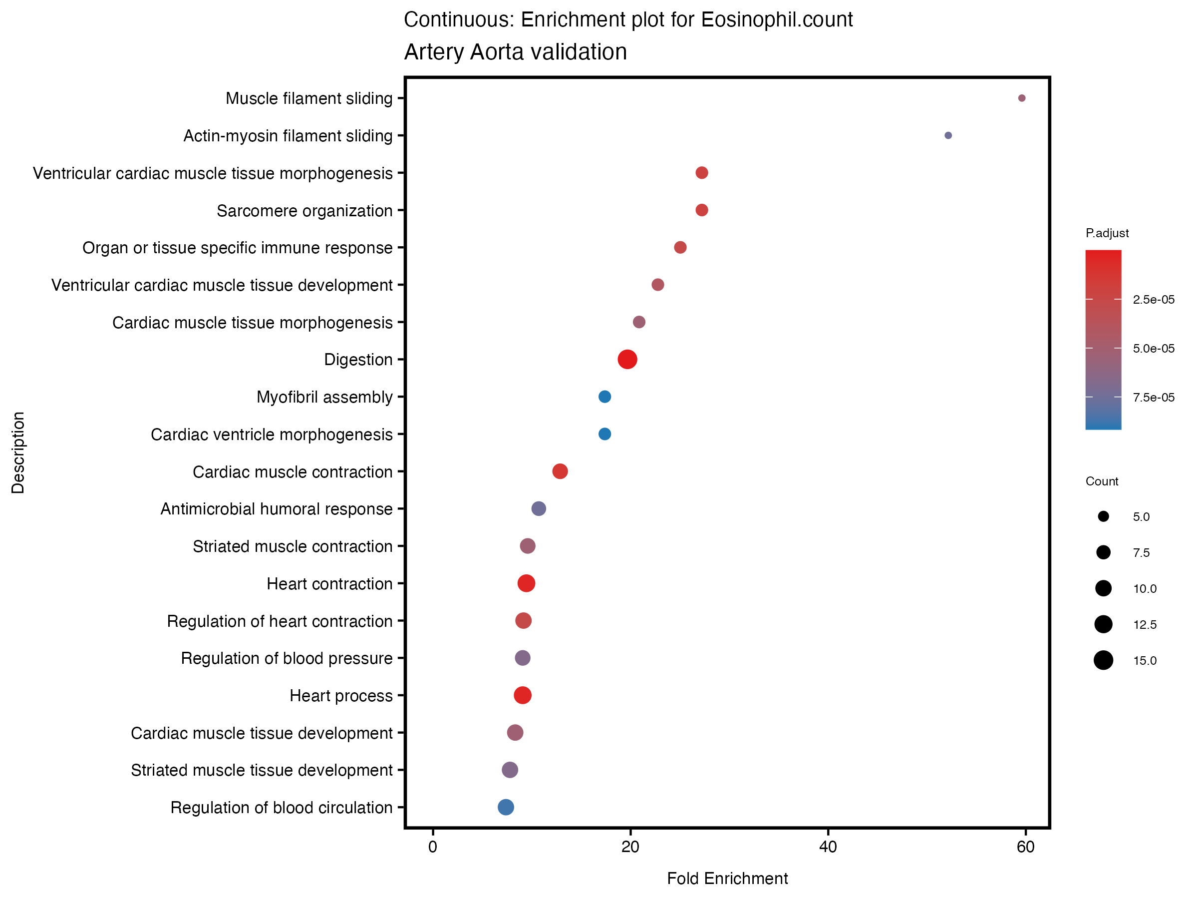
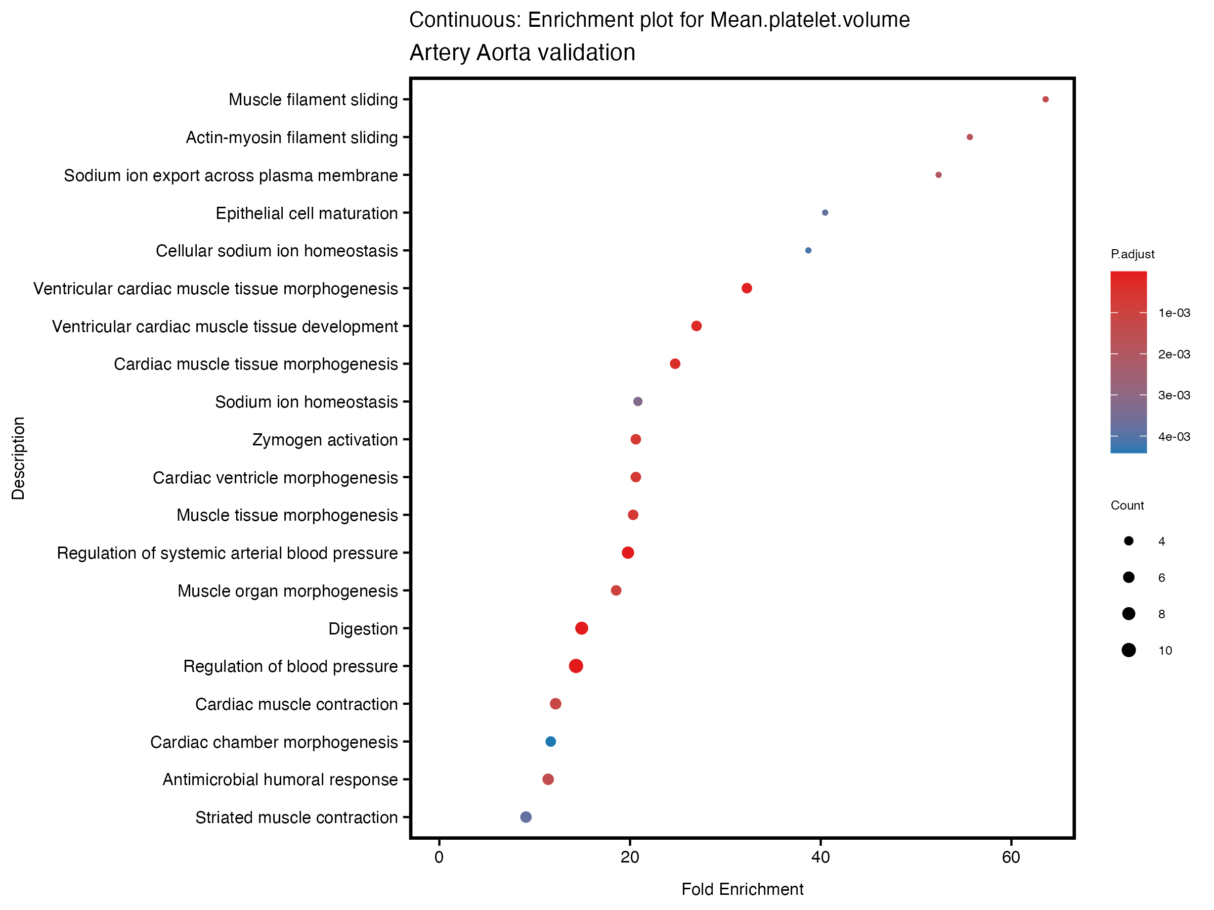
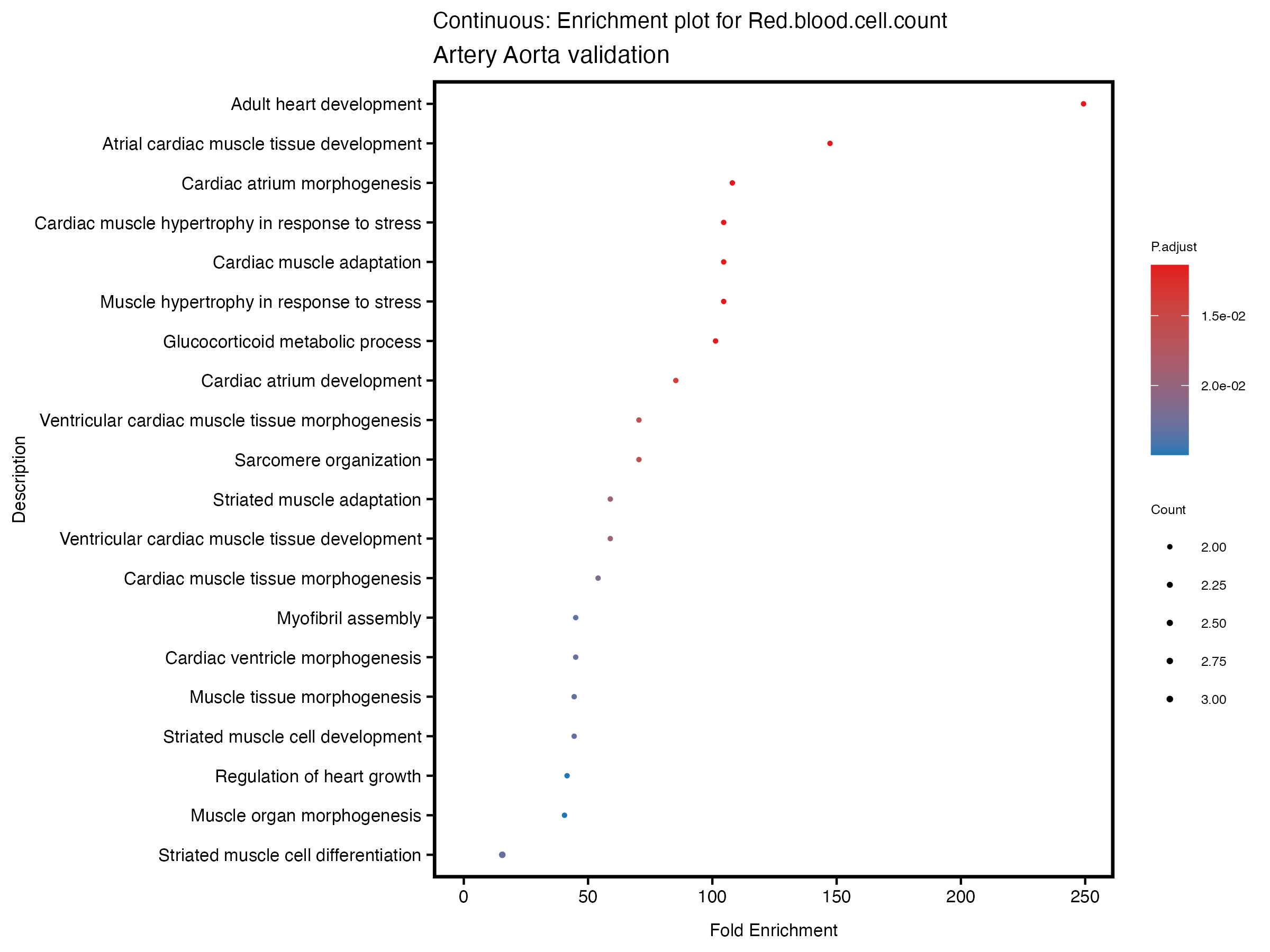
  if (nrow(gse) >= 20) {
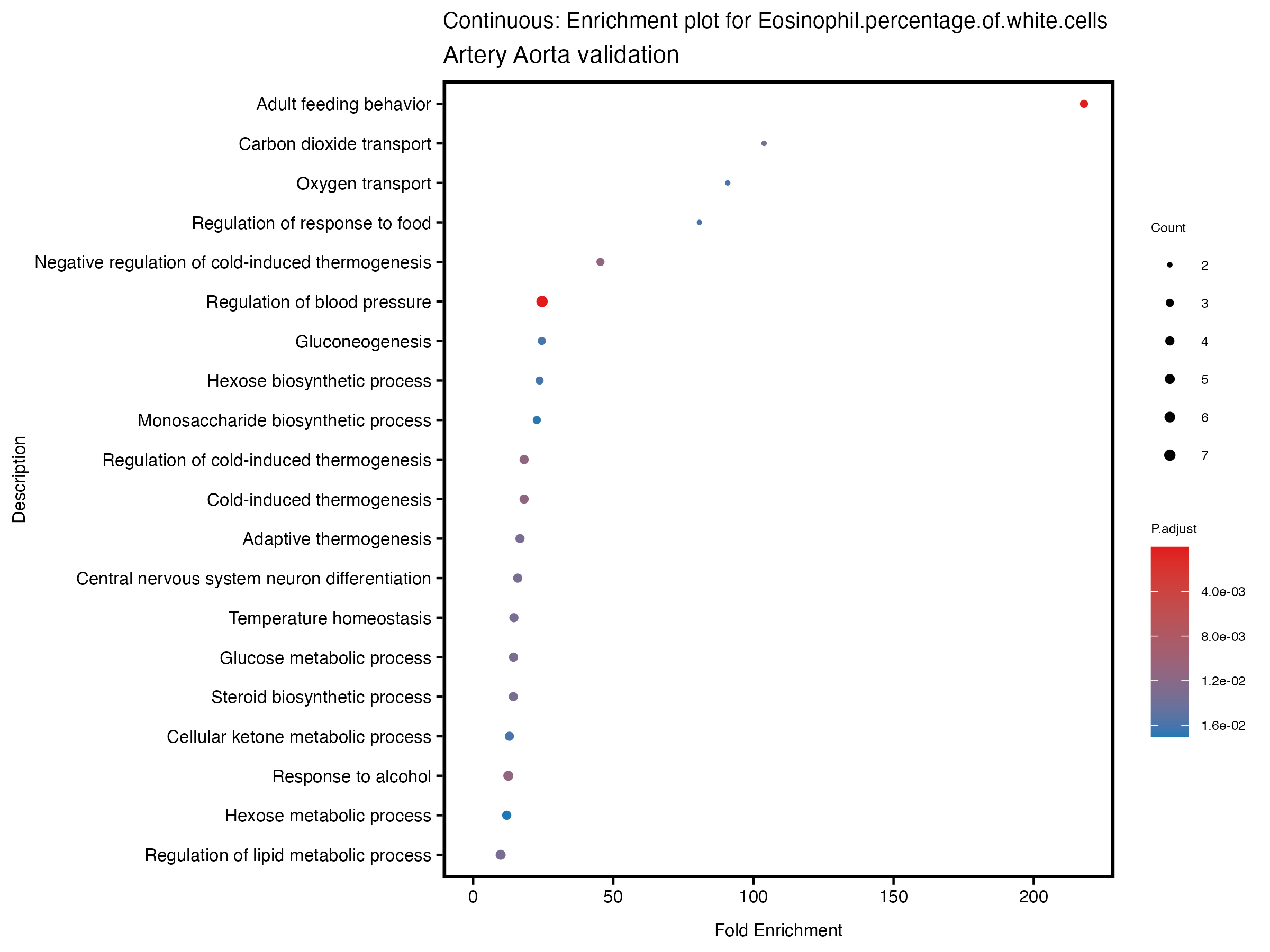
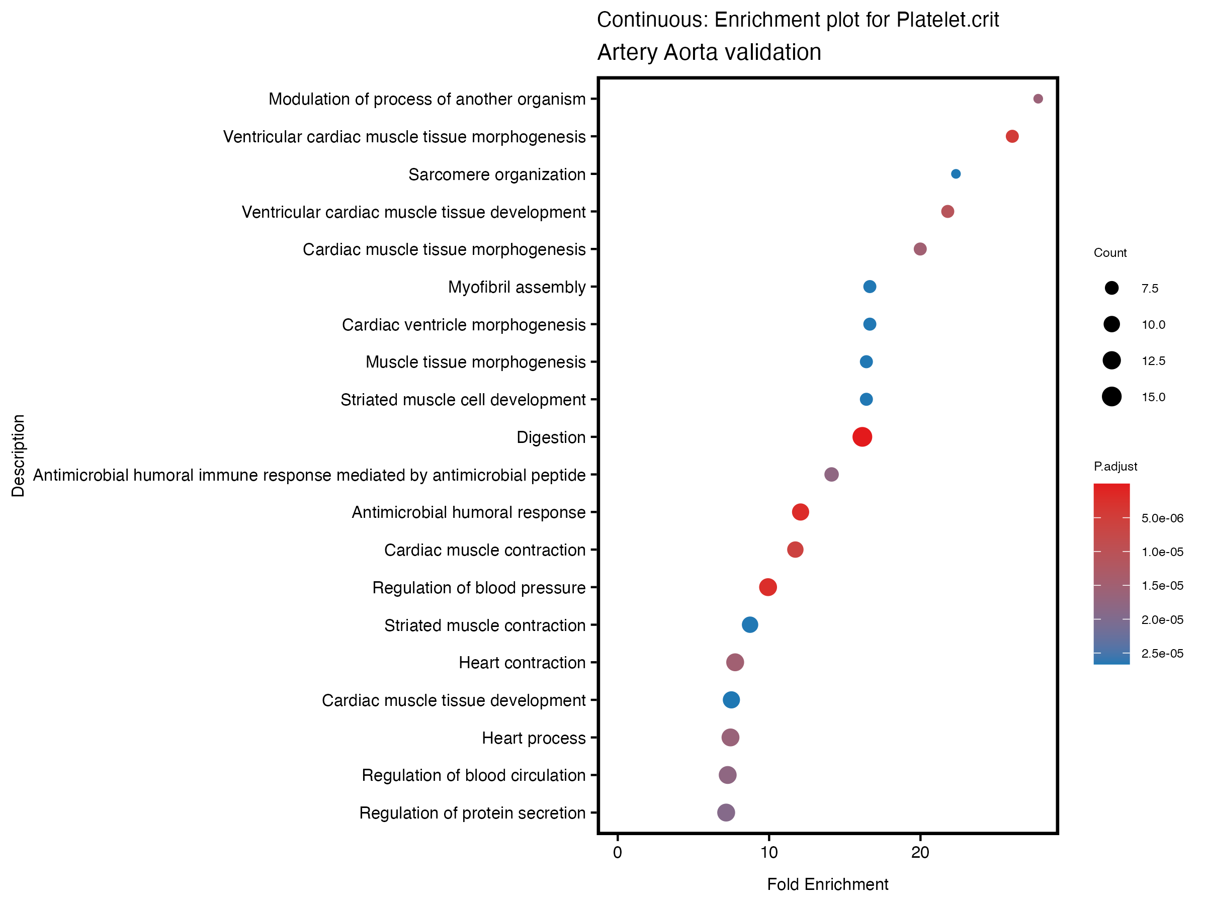
    enrich_plot <- plotEnrich(gse[1:20,], plot_type = "dot", scale_ratio = 0.5) +
    labs(title = paste("Continuous: Enrichment plot for", trait), 
         subtitle = "Artery Aorta validation") + 
    theme(plot.title = element_text(size = 10)) 
  }else{
    enrich_plot <- plotEnrich(gse, plot_type = "dot", scale_ratio = 0.5) +
    labs(title = paste("Continuous: Enrichment plot for", trait), 
         subtitle = "Artery Aorta validation") + 
    theme(plot.title = element_text(size = 10)) 
  }
  ggsave(paste0("enrichment_plot_", trait, "_artery_validation.png"), plot = enrich_plot, width = 8, height = 6)
}

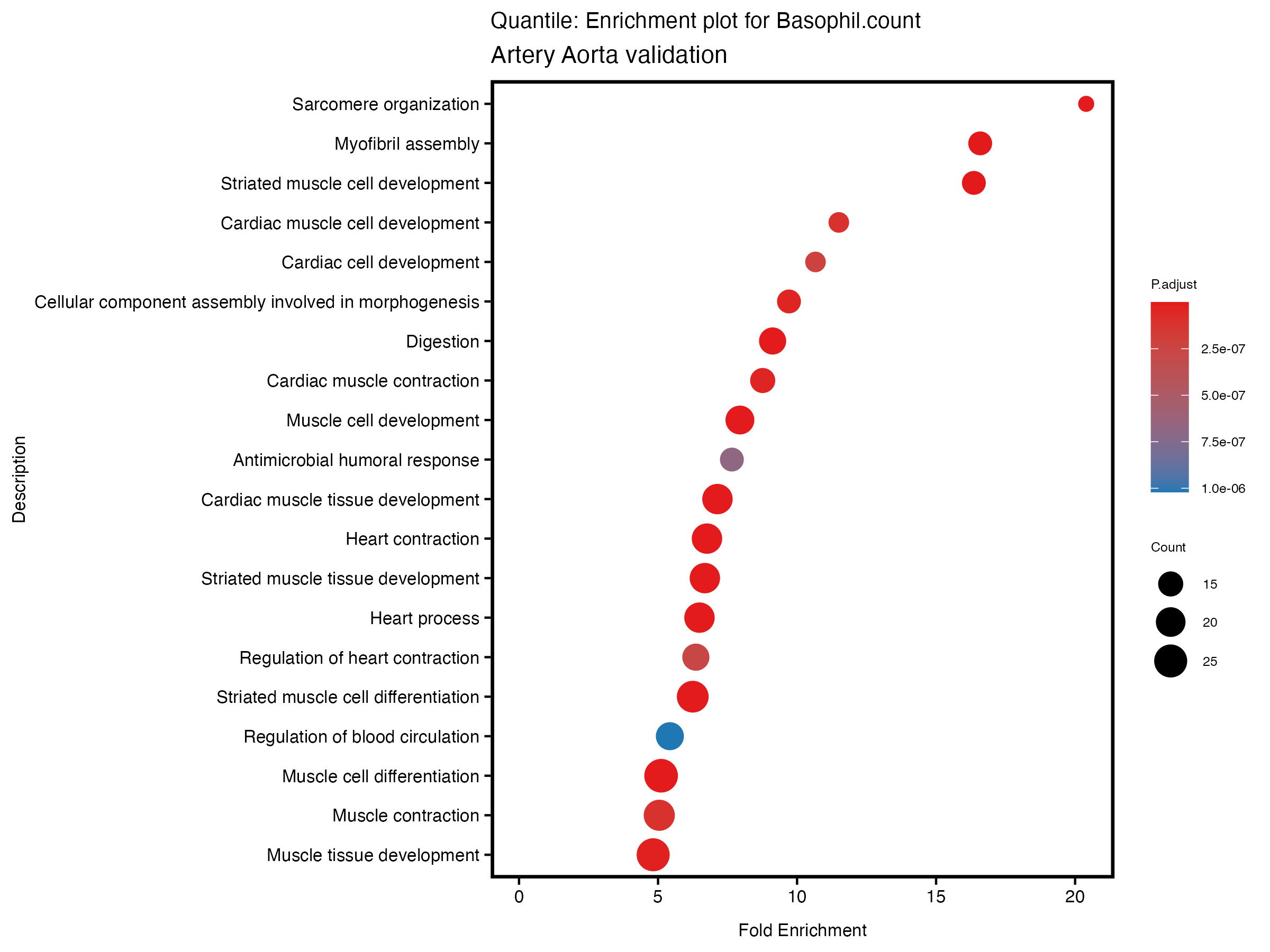
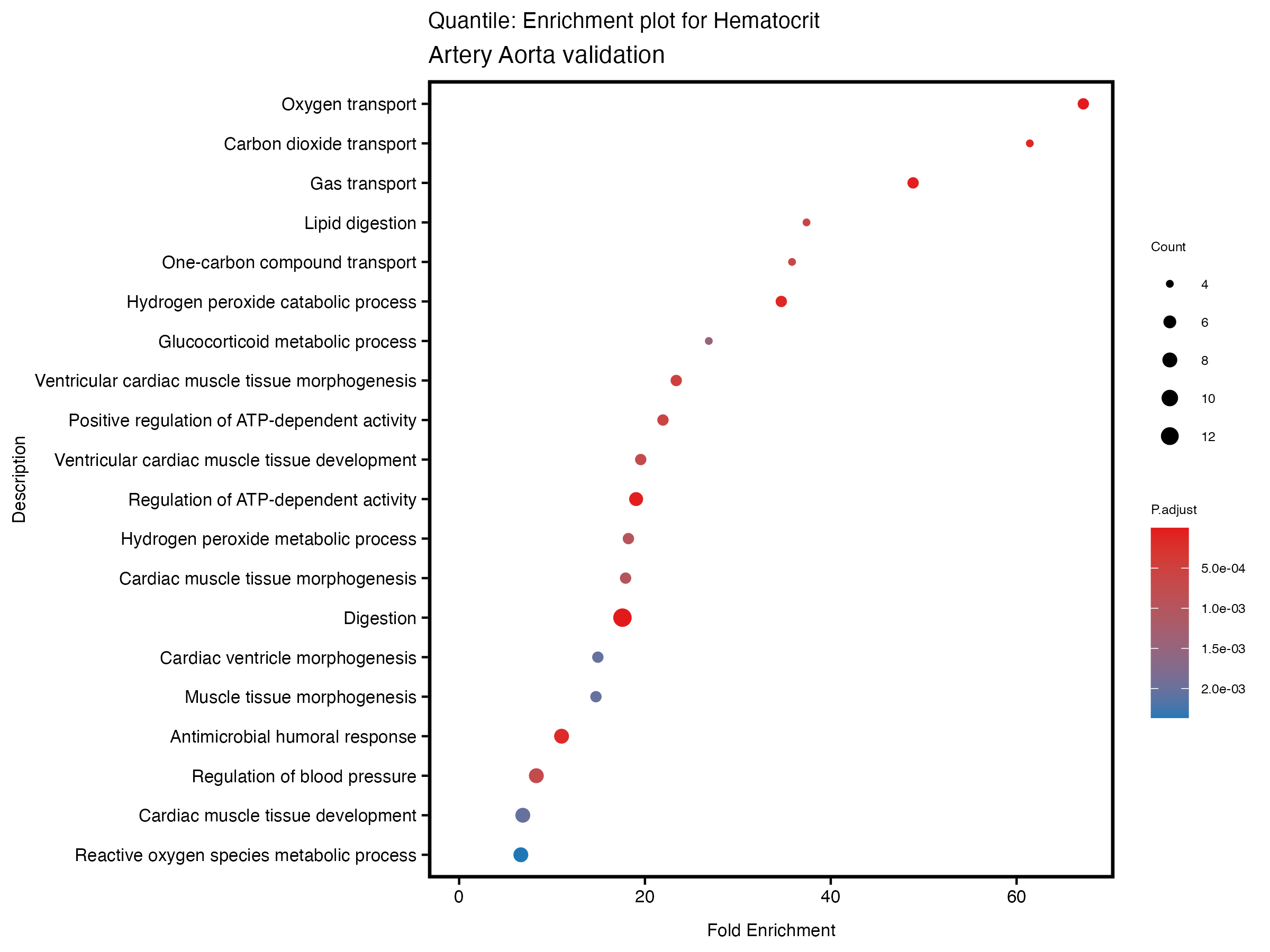
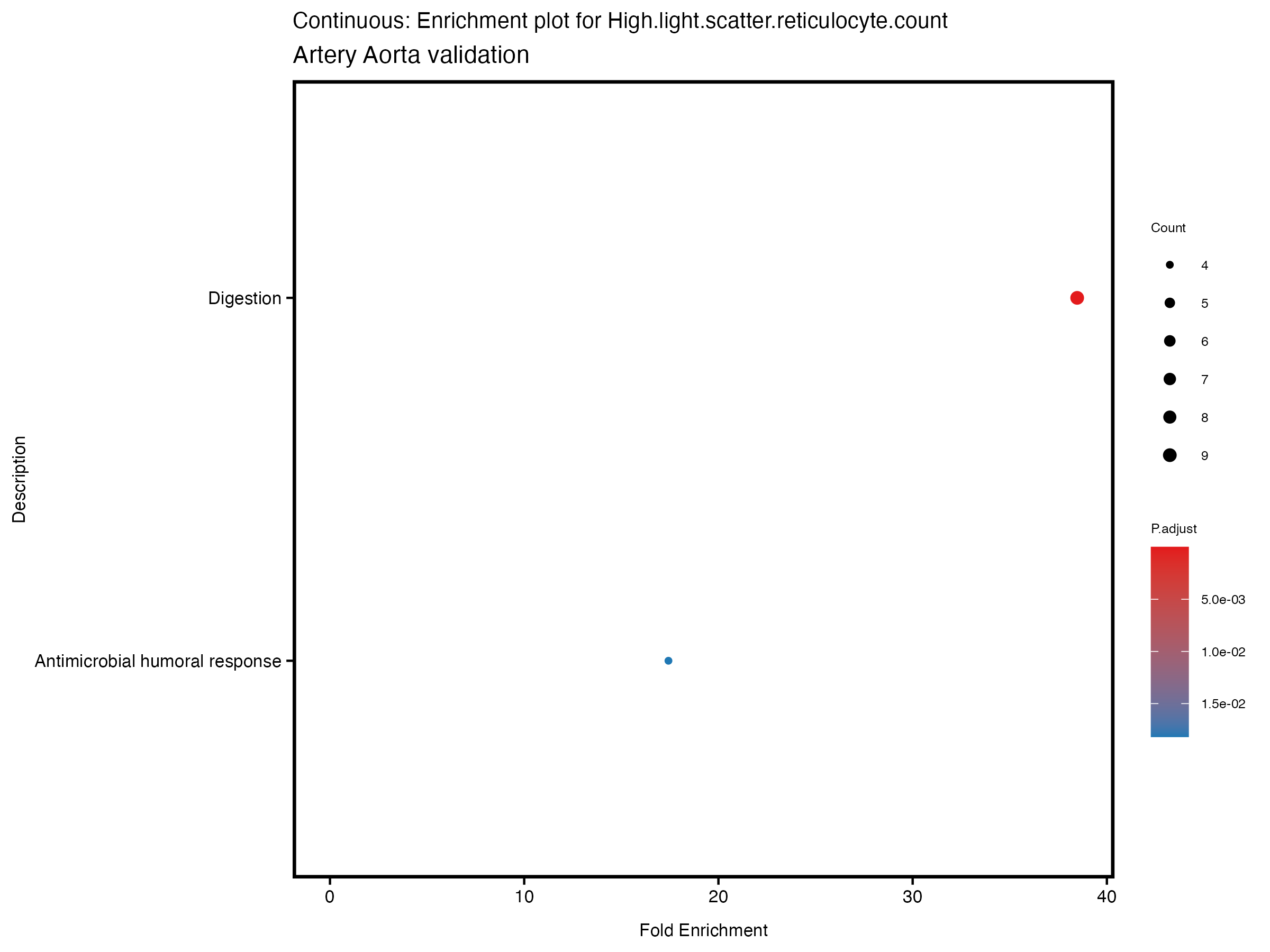
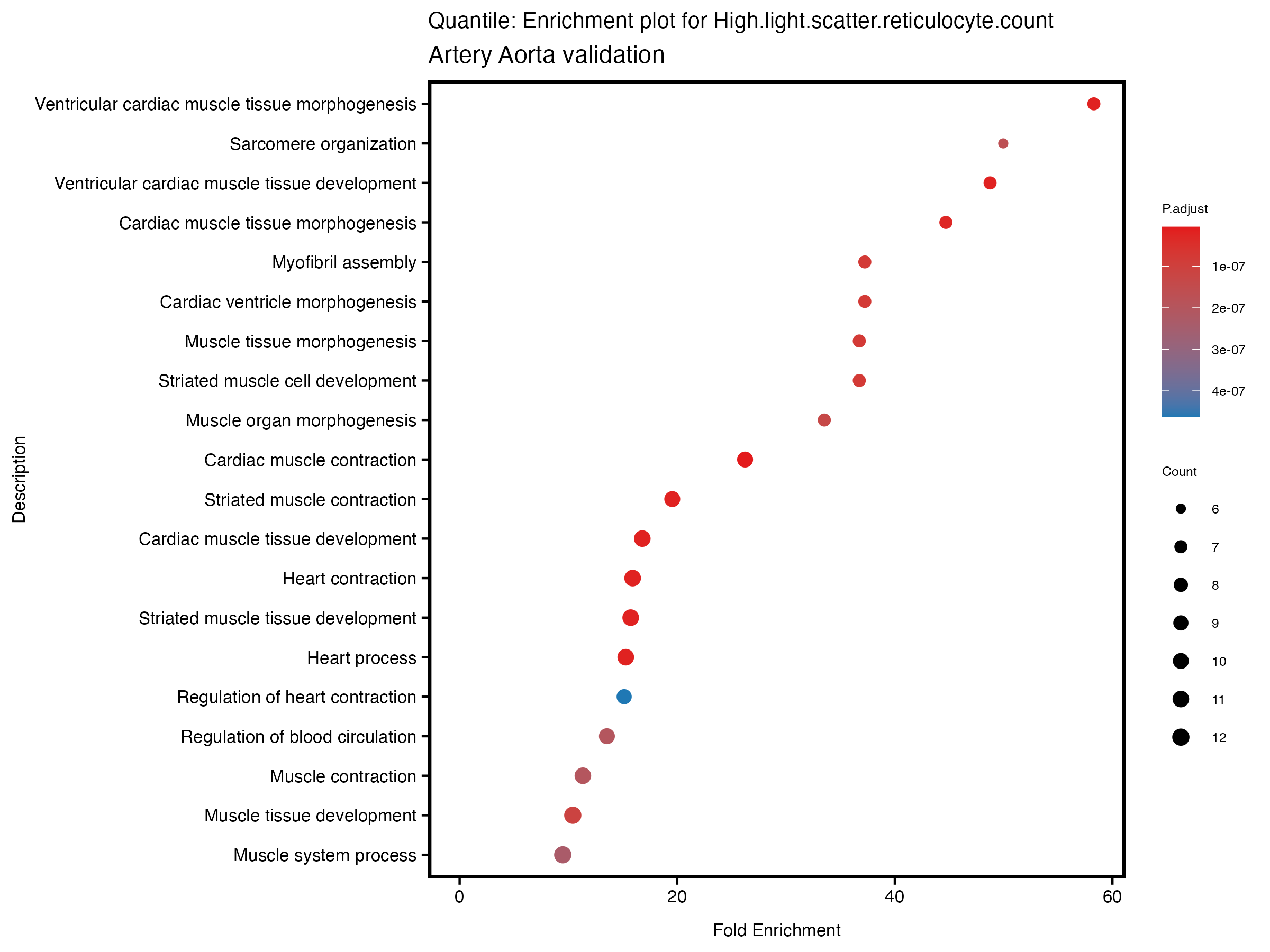
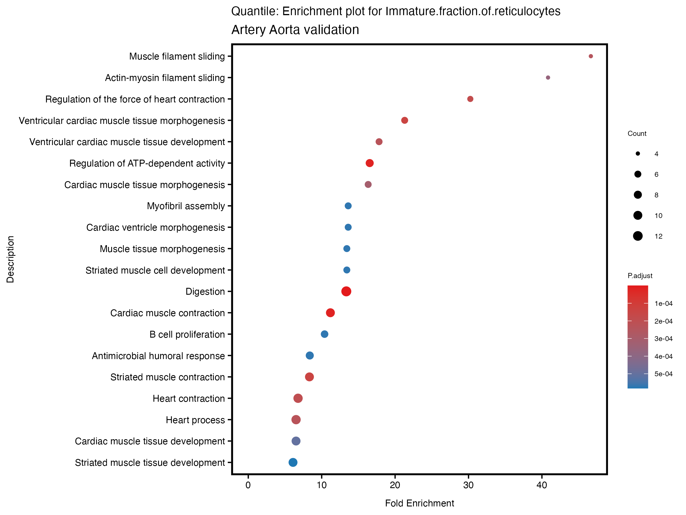
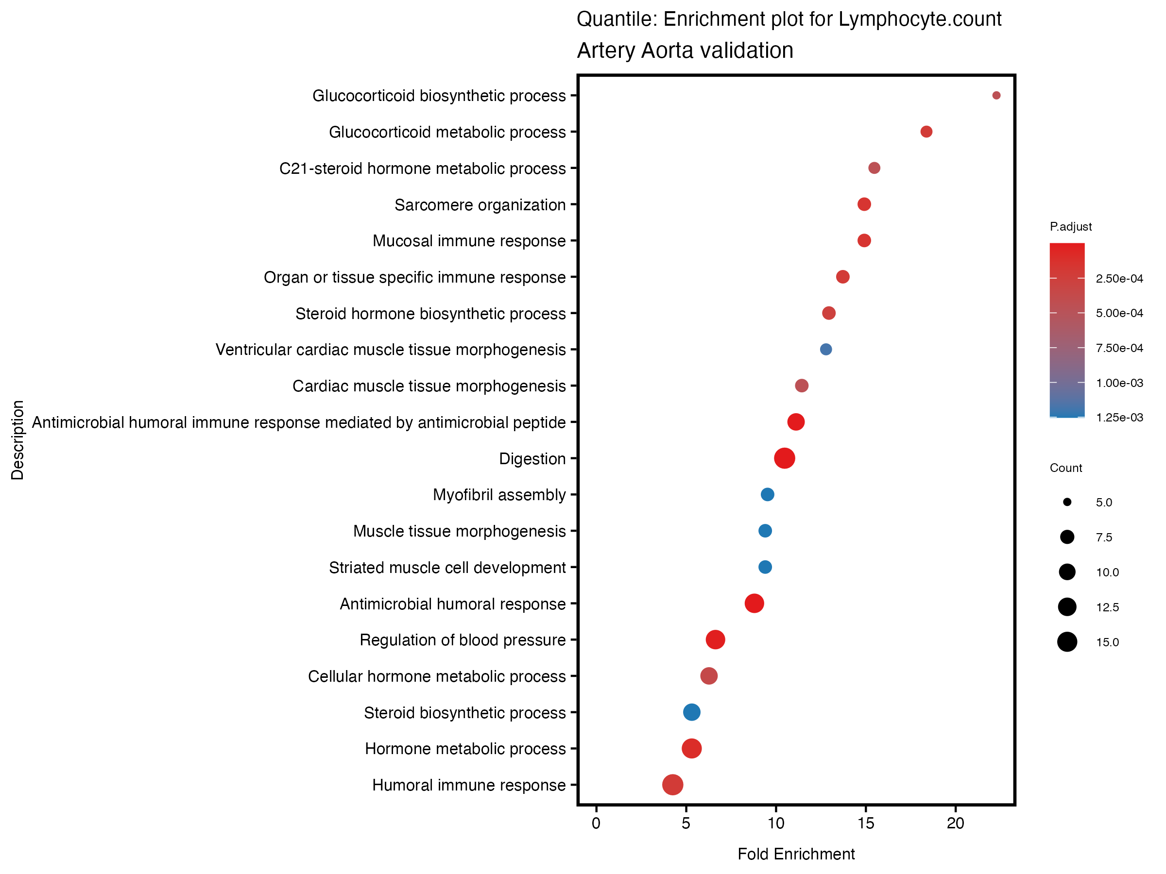
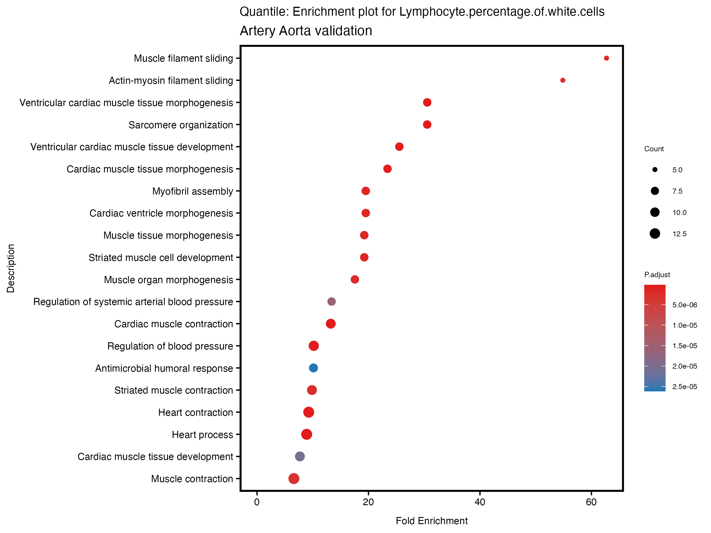
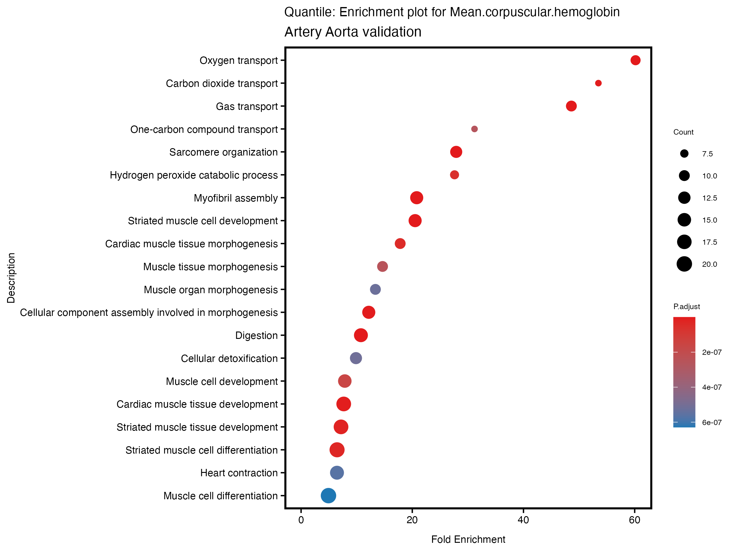
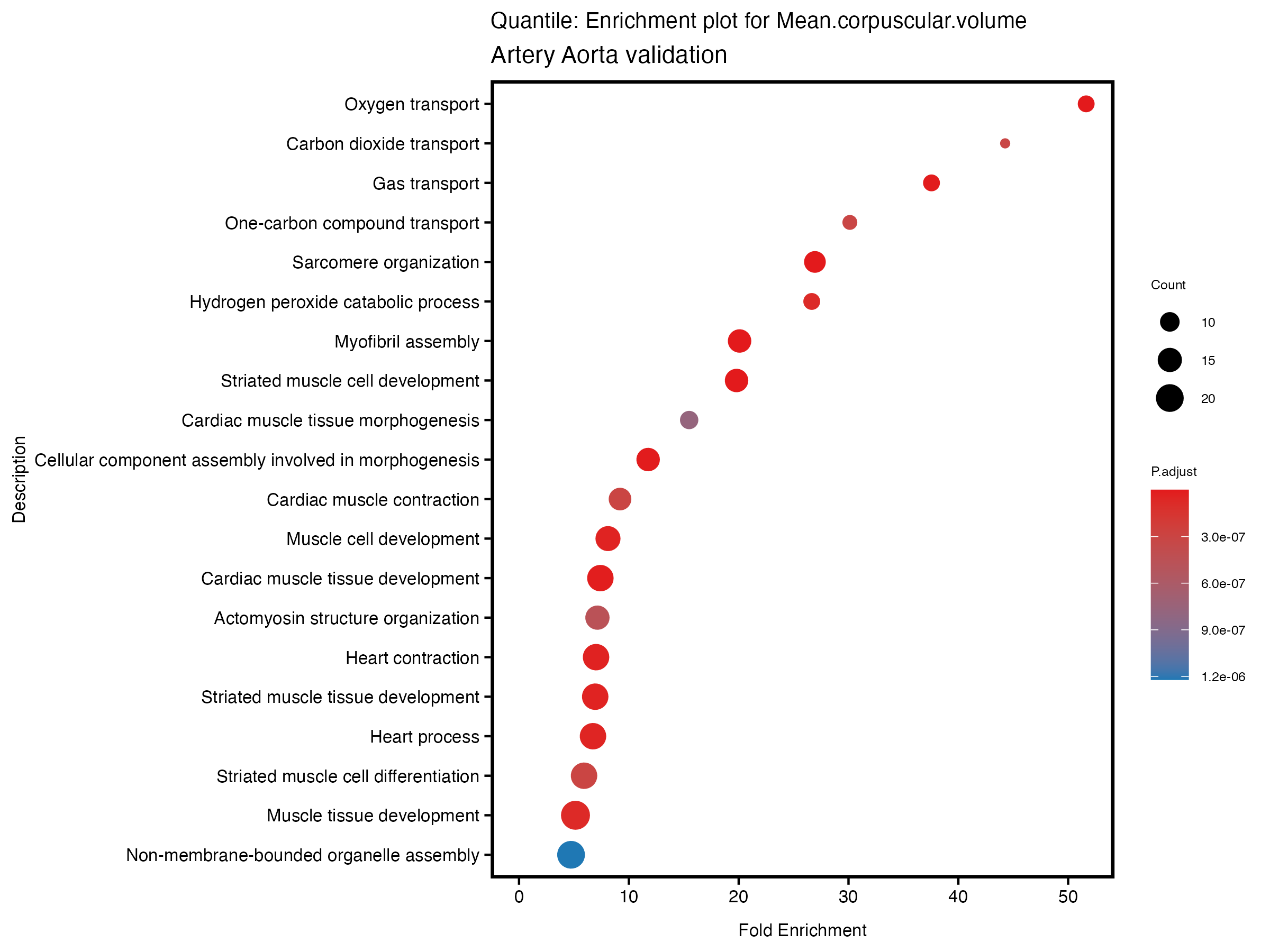
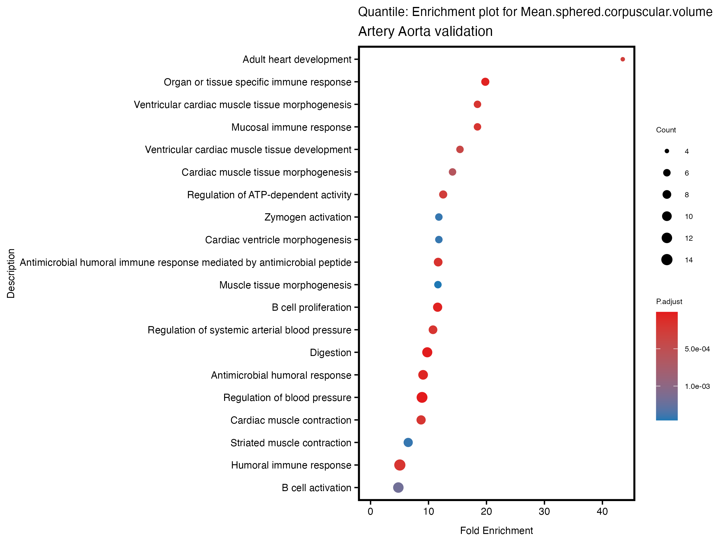
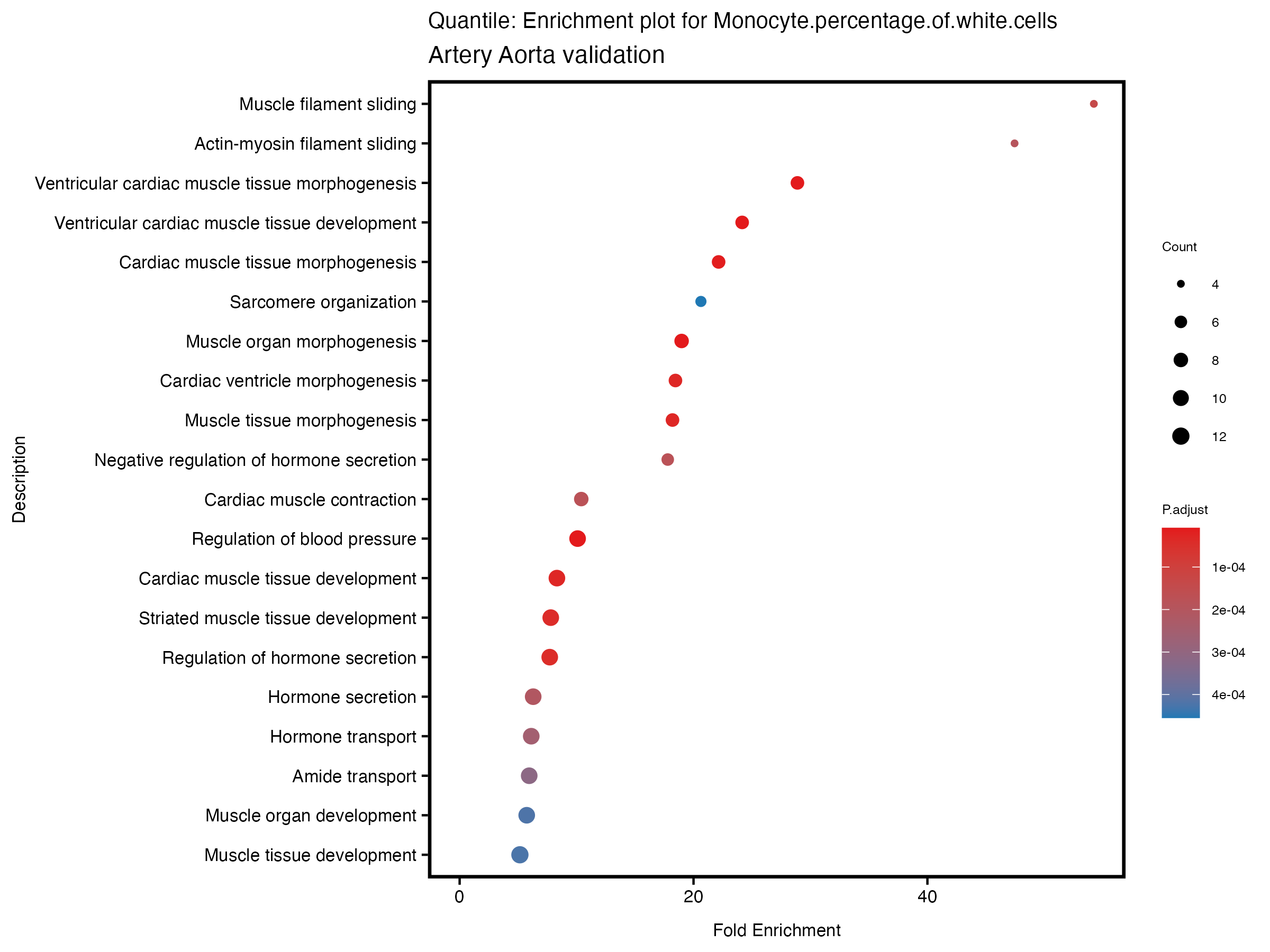
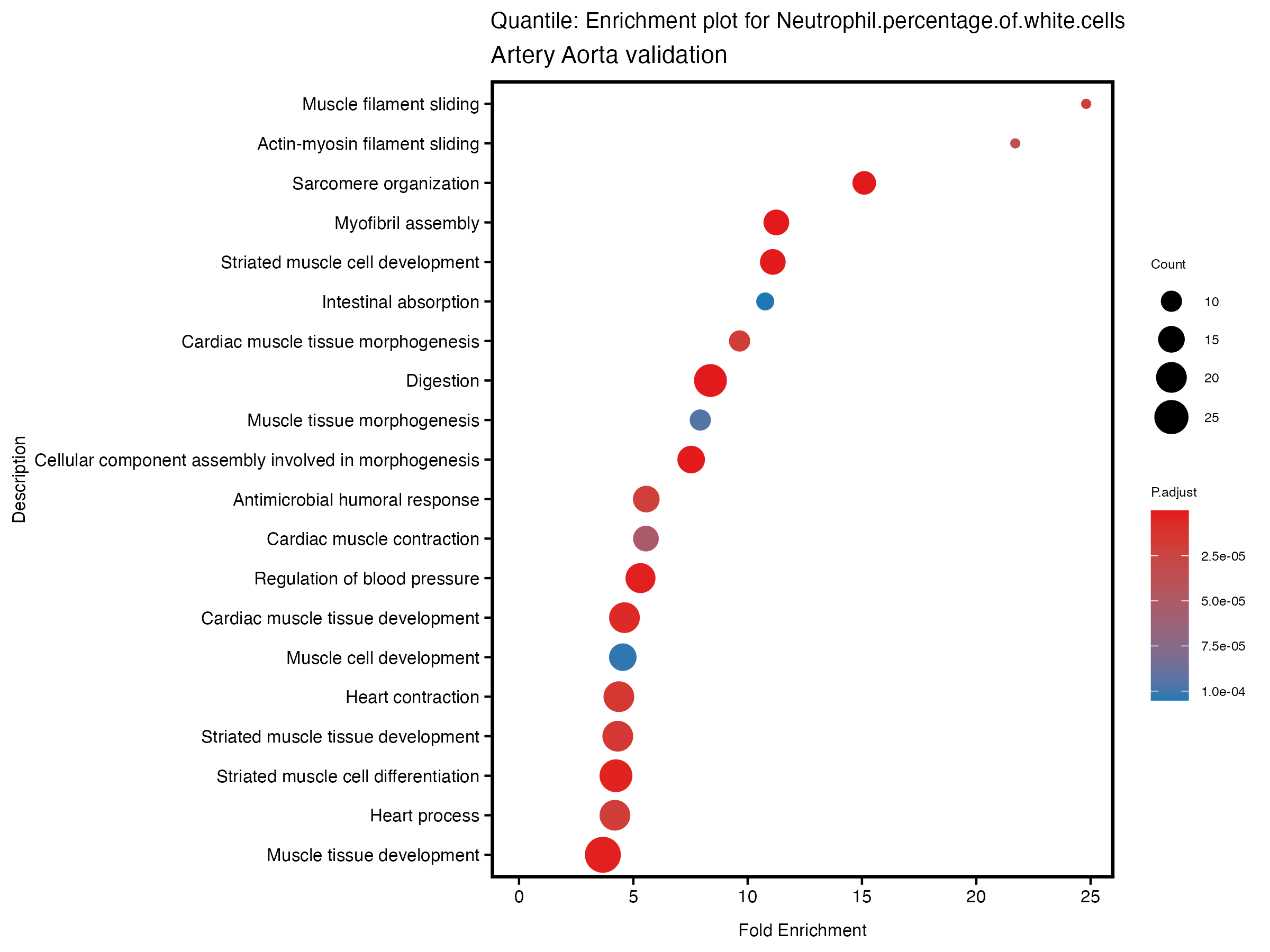
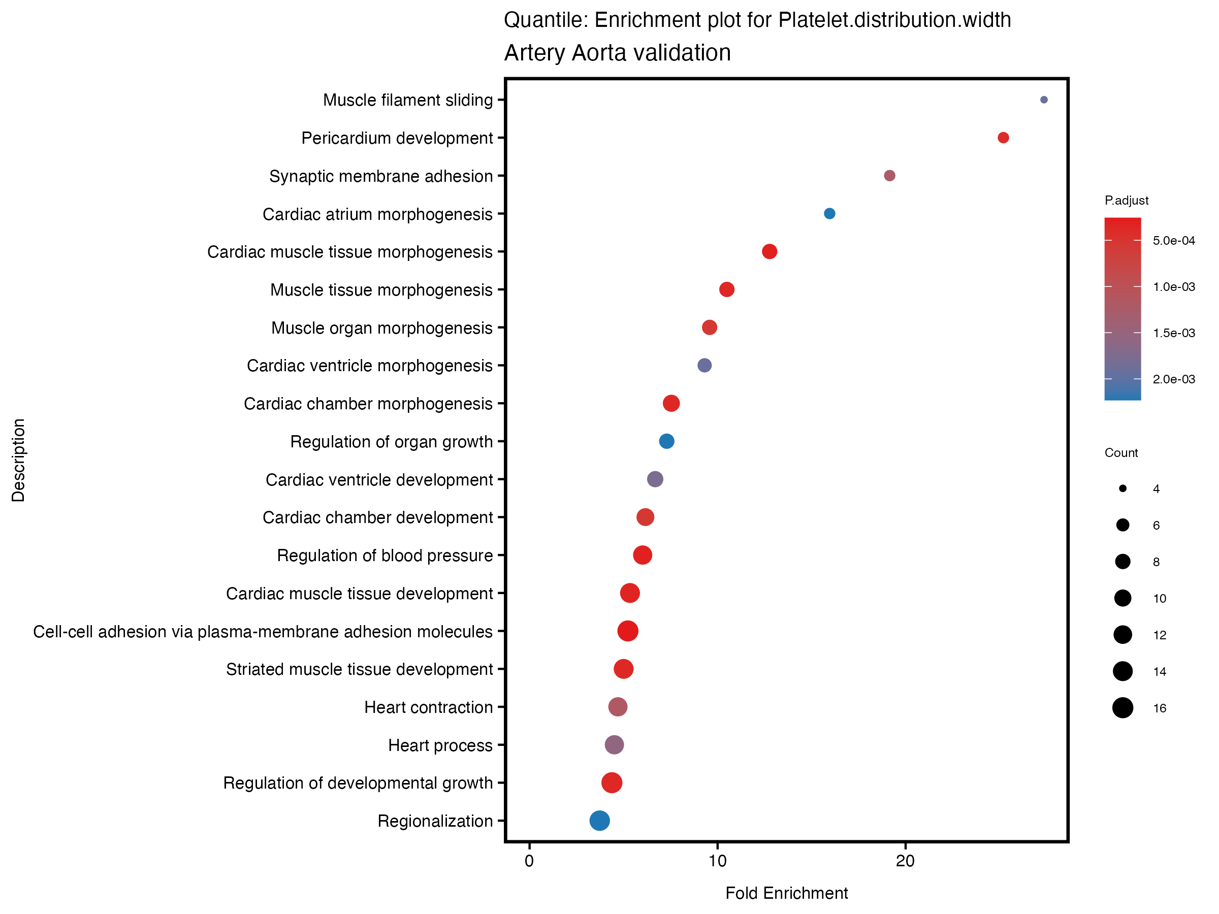
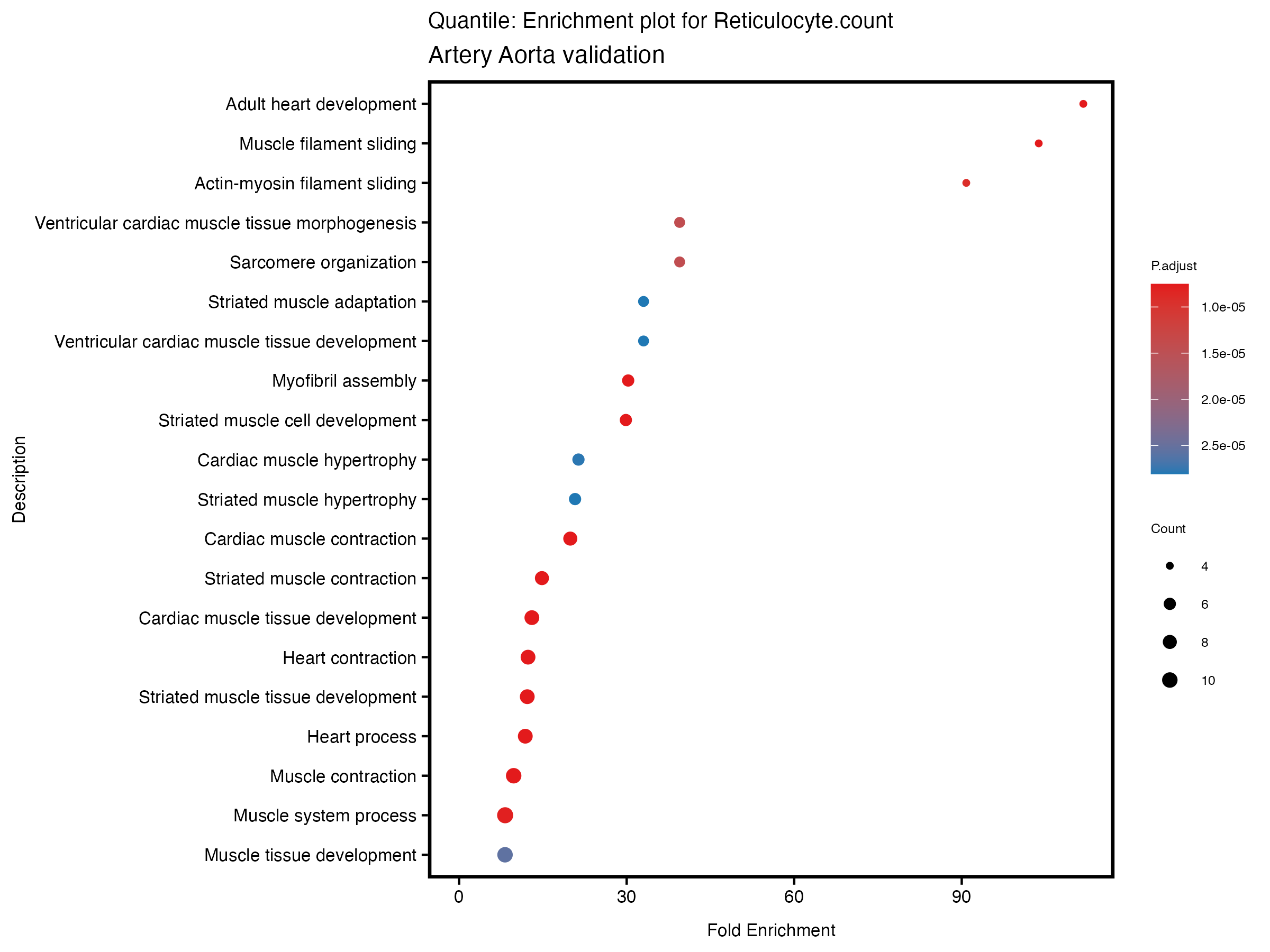
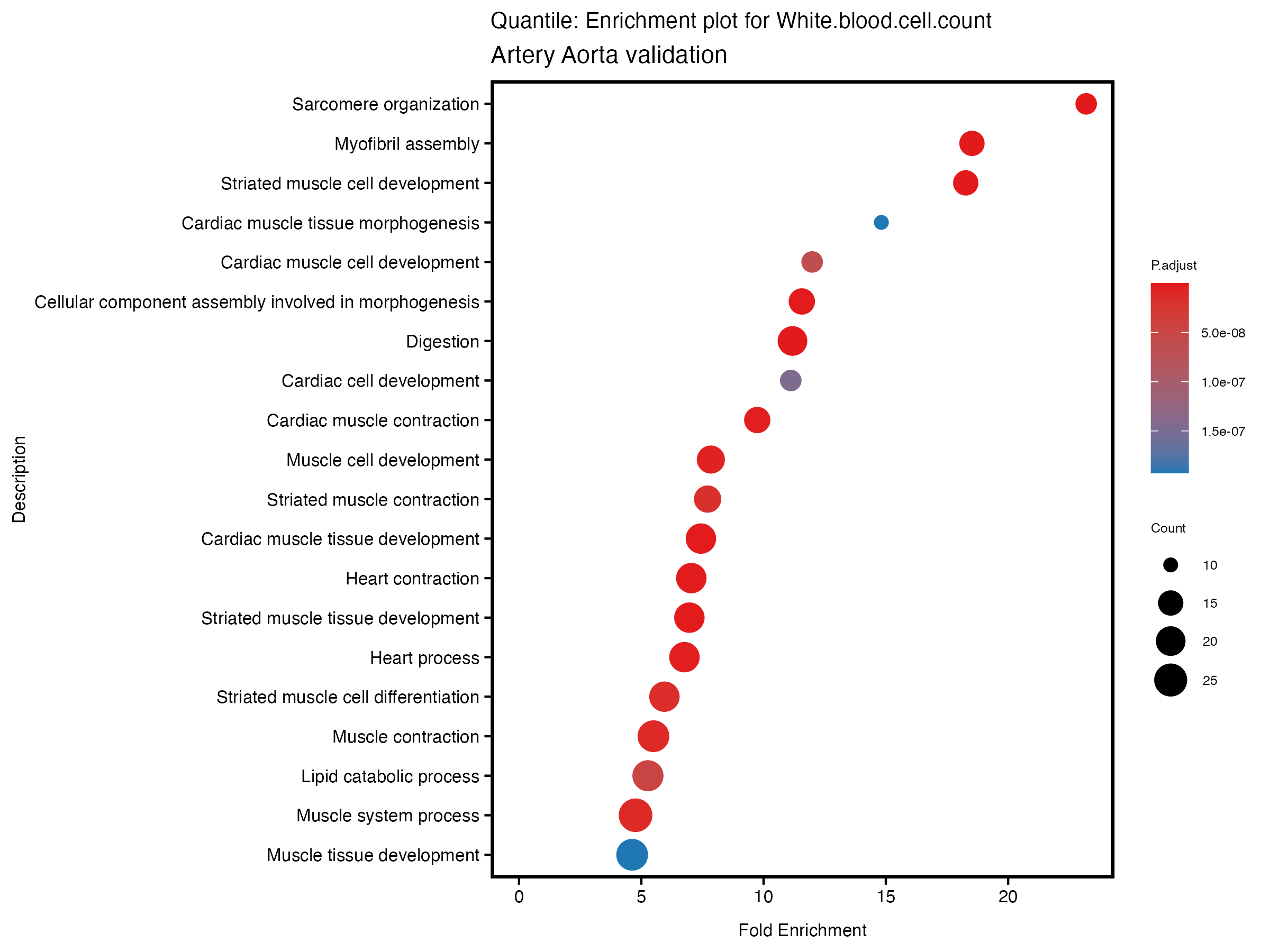
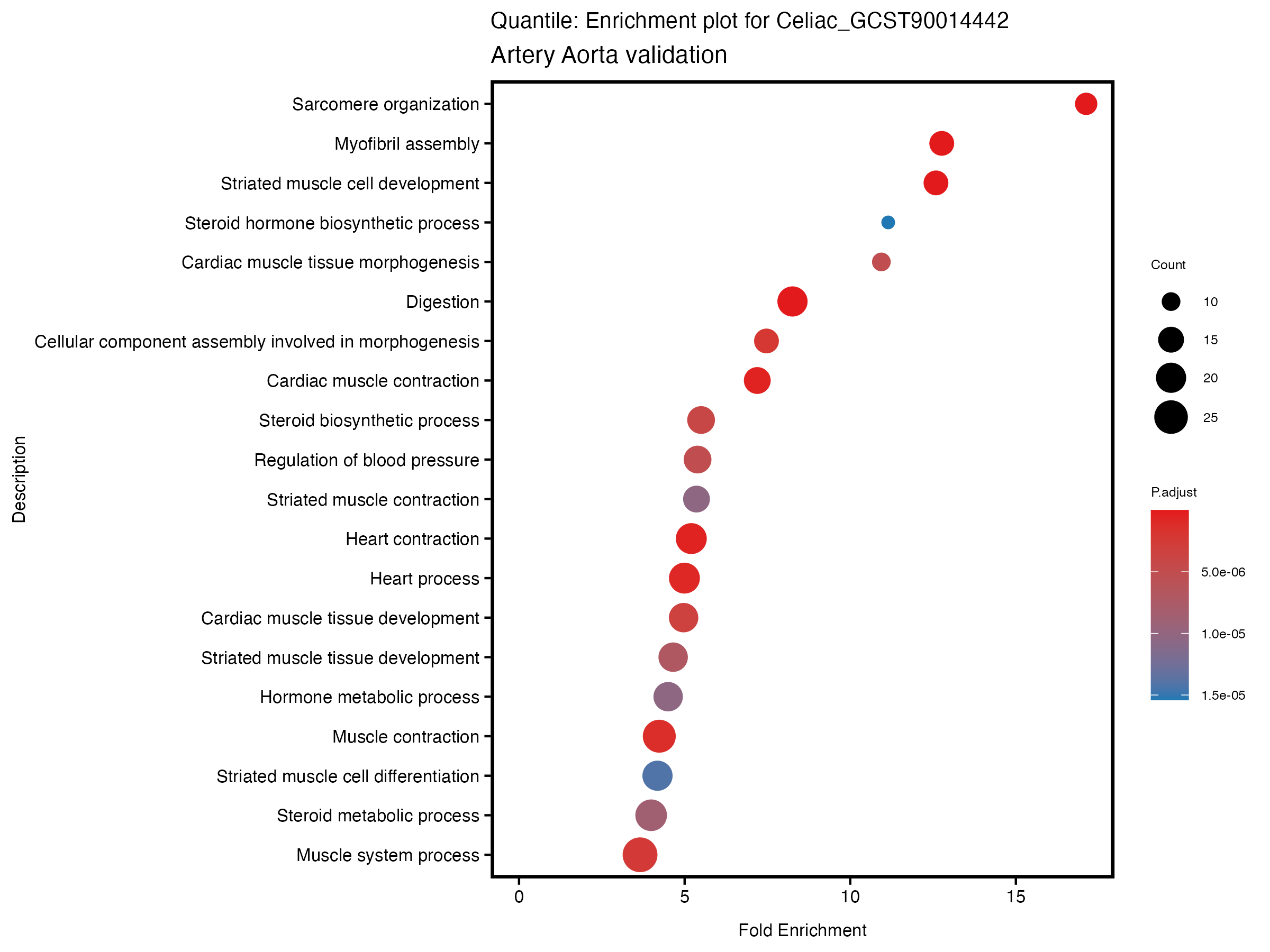
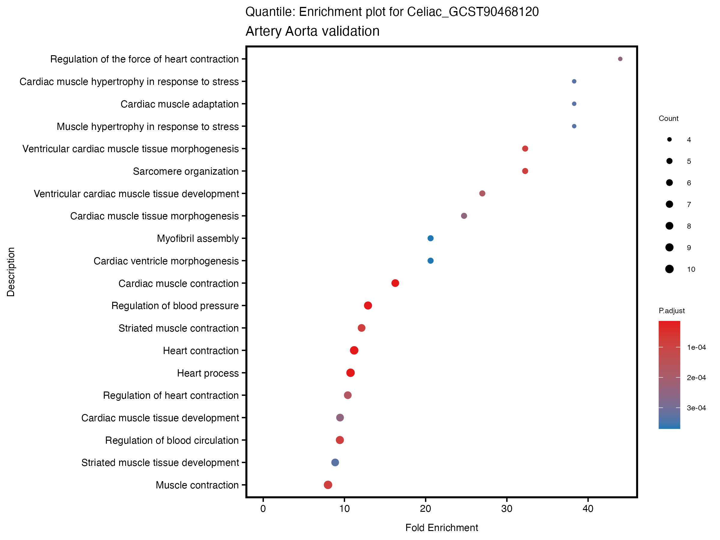
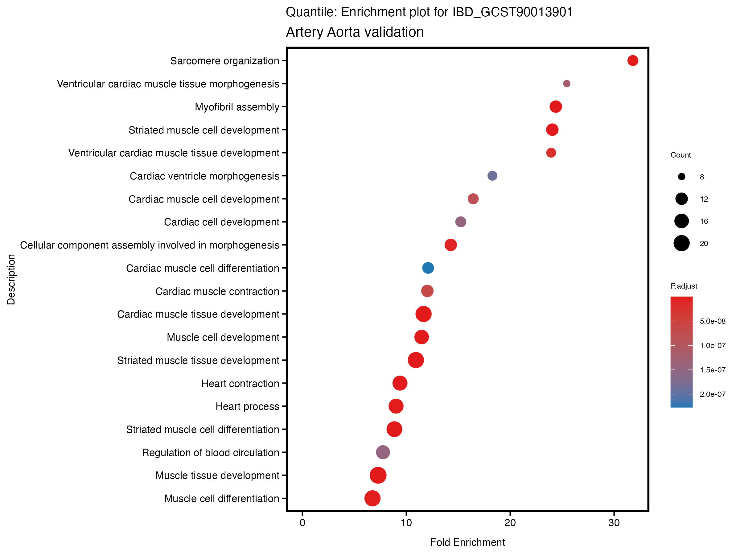
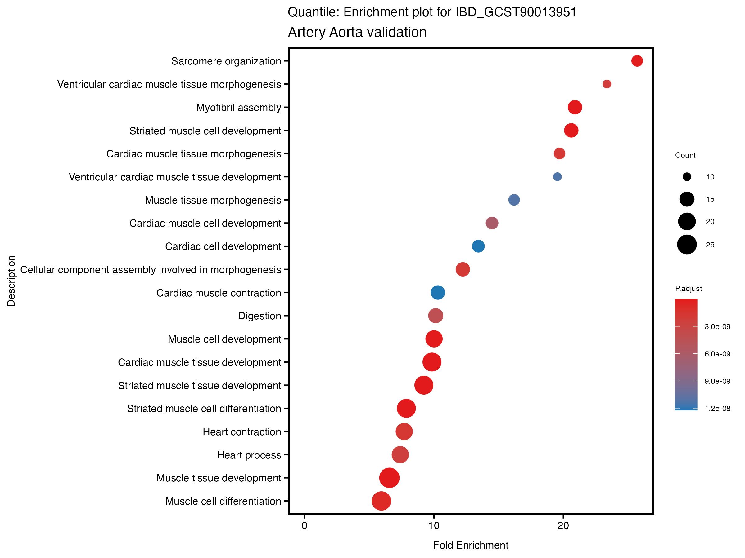
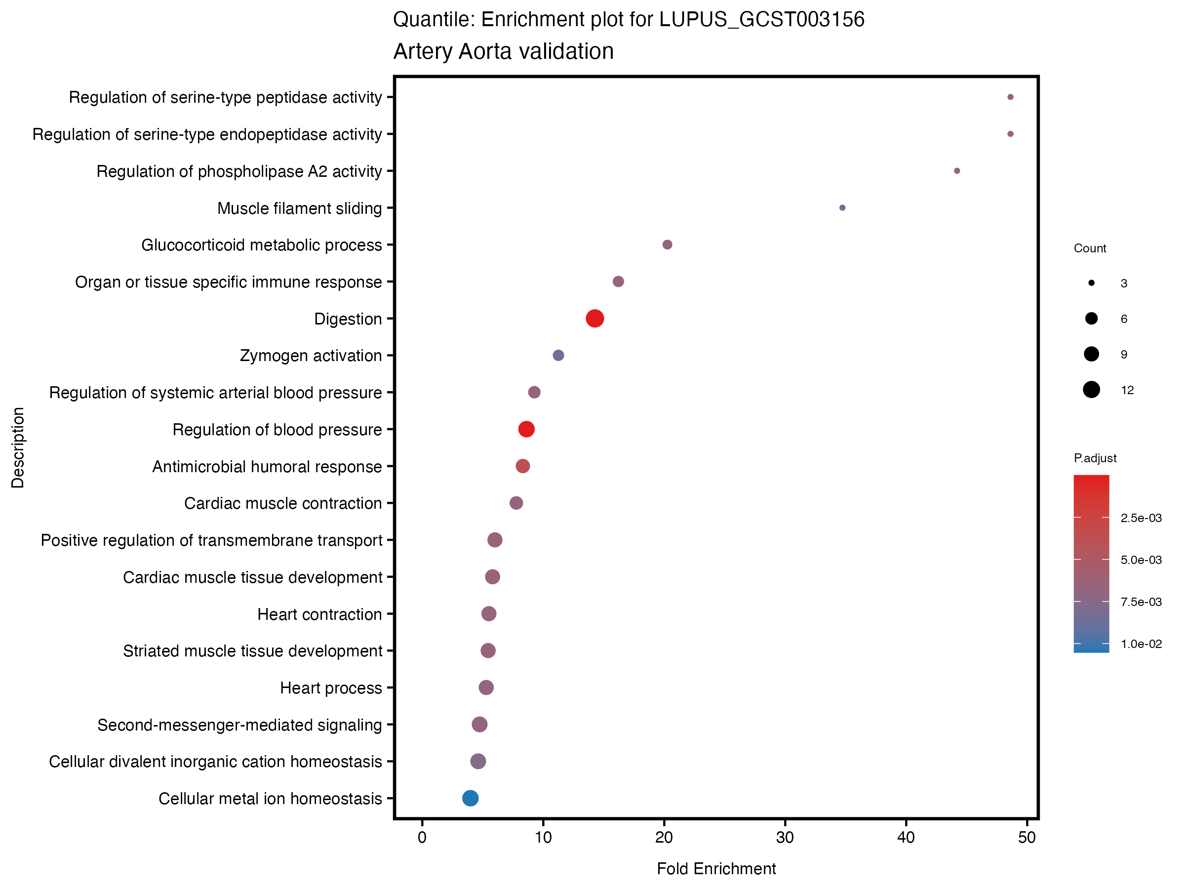
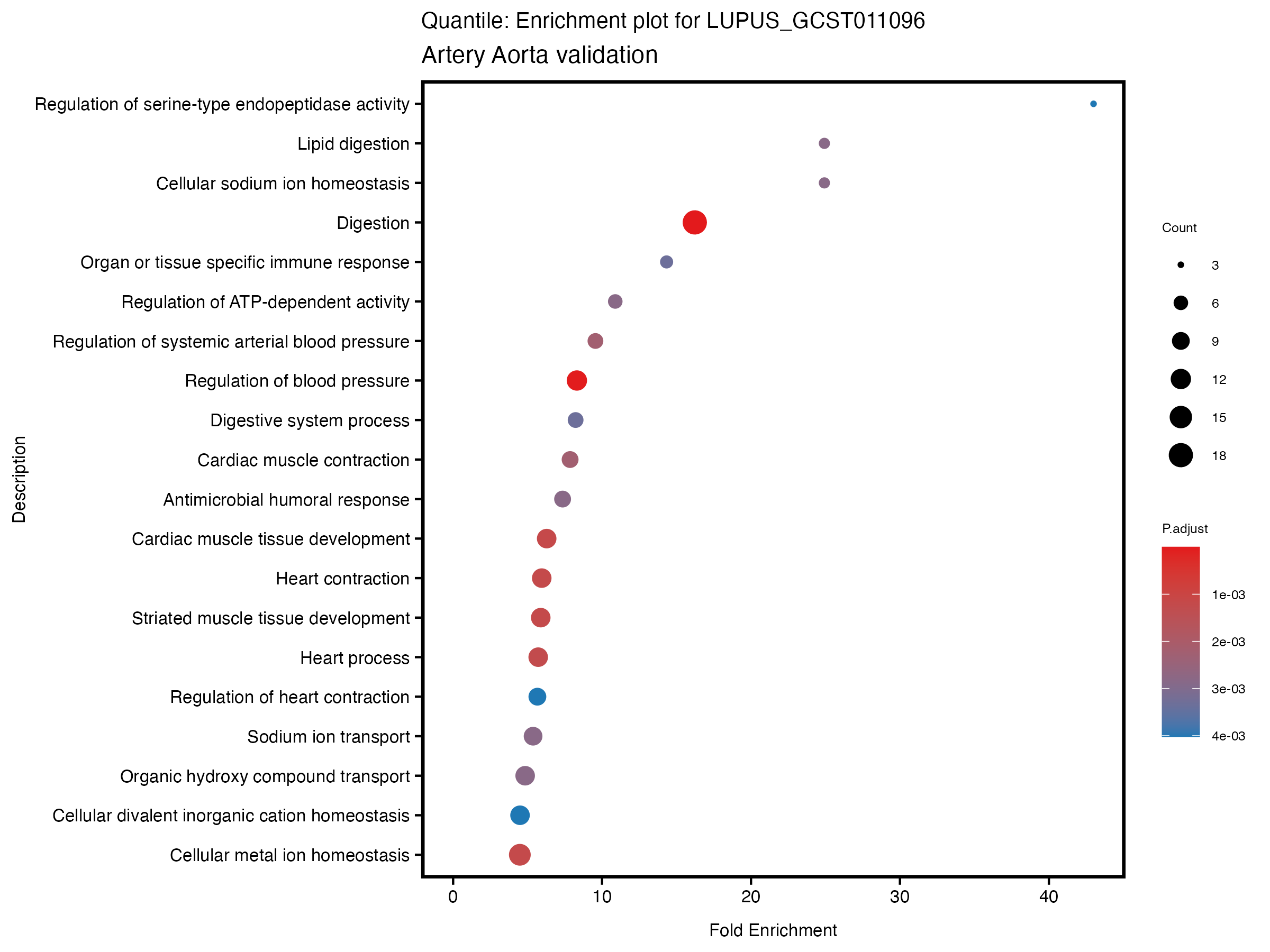
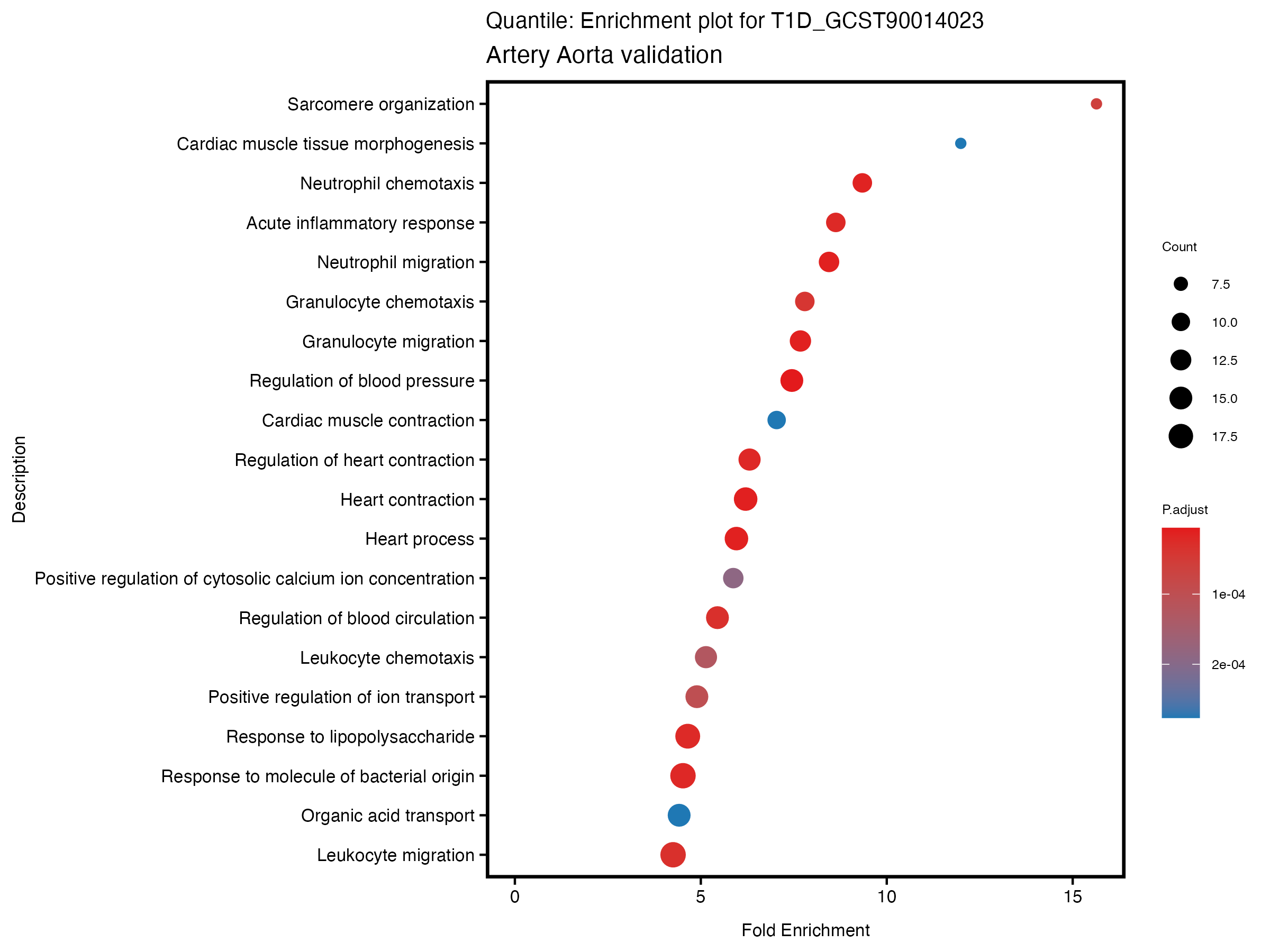
# quantile
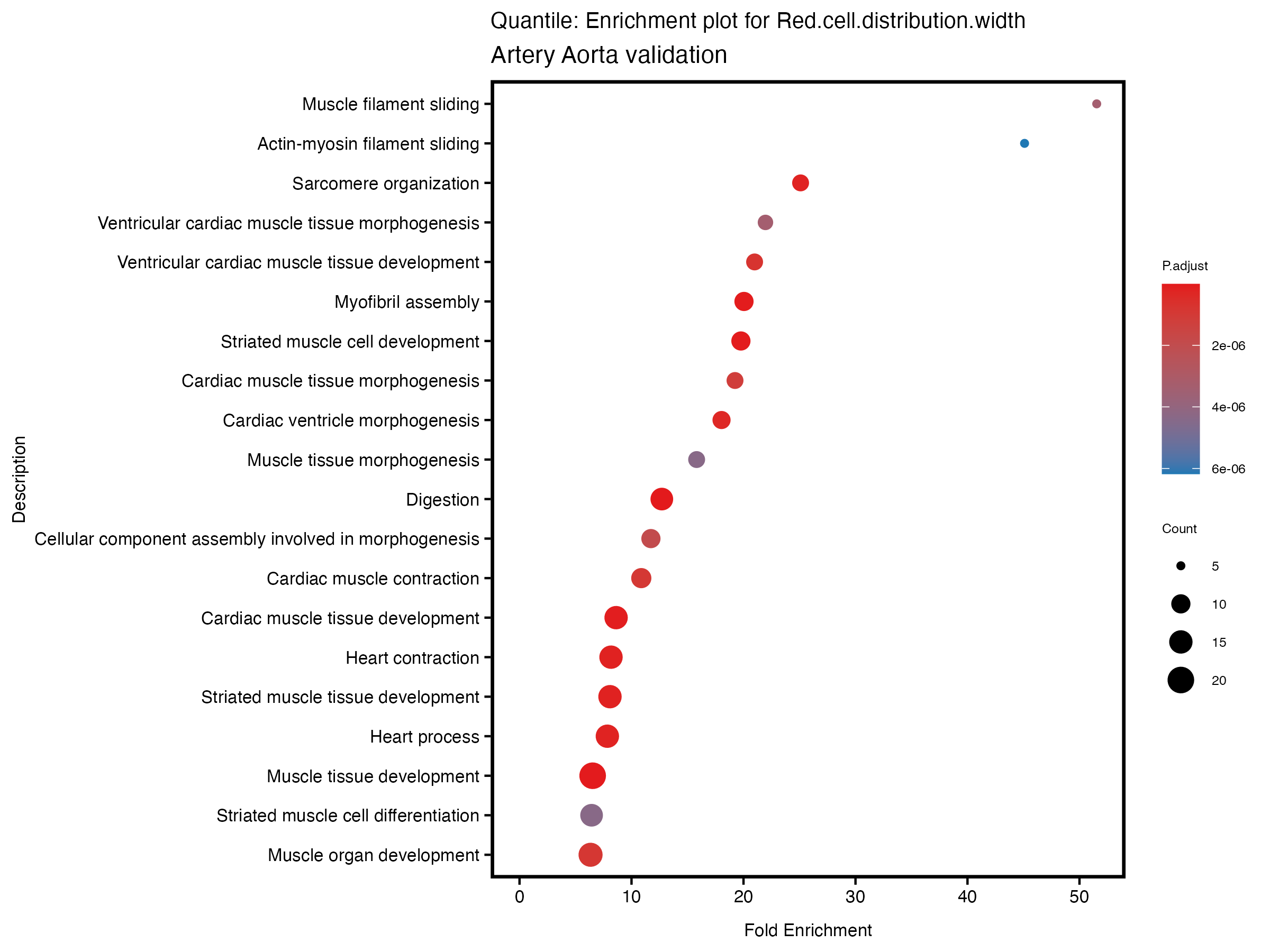
dir_path <- "analysis/quantile_artery"
files <- list.files(dir_path, pattern = "differential_expression_.*_quantile_results_artery_validation.csv",
                    full.names = TRUE)

for (file in files) {
  trait <- gsub("differential_expression_(.*)_quantile_results_artery_validation.csv", "\\1", basename(file))
  trait
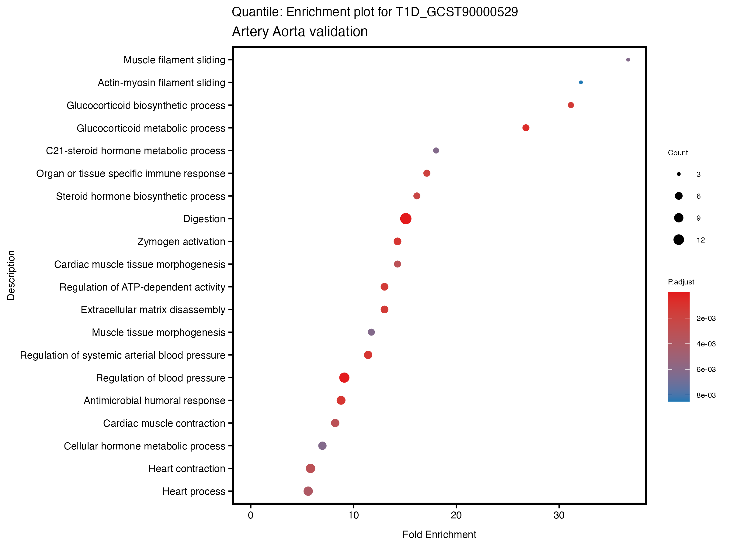
  res_tableOE <- read.csv(file, header = T, row.names = 1)
  
  deGenes <- res_tableOE[res_tableOE$padj < 0.1 & 
                           abs(res_tableOE$log2FoldChange) >= 0.5, ]
  deGenes$gene_id <- gsub("\\.\\d+$", "", rownames(deGenes))
  
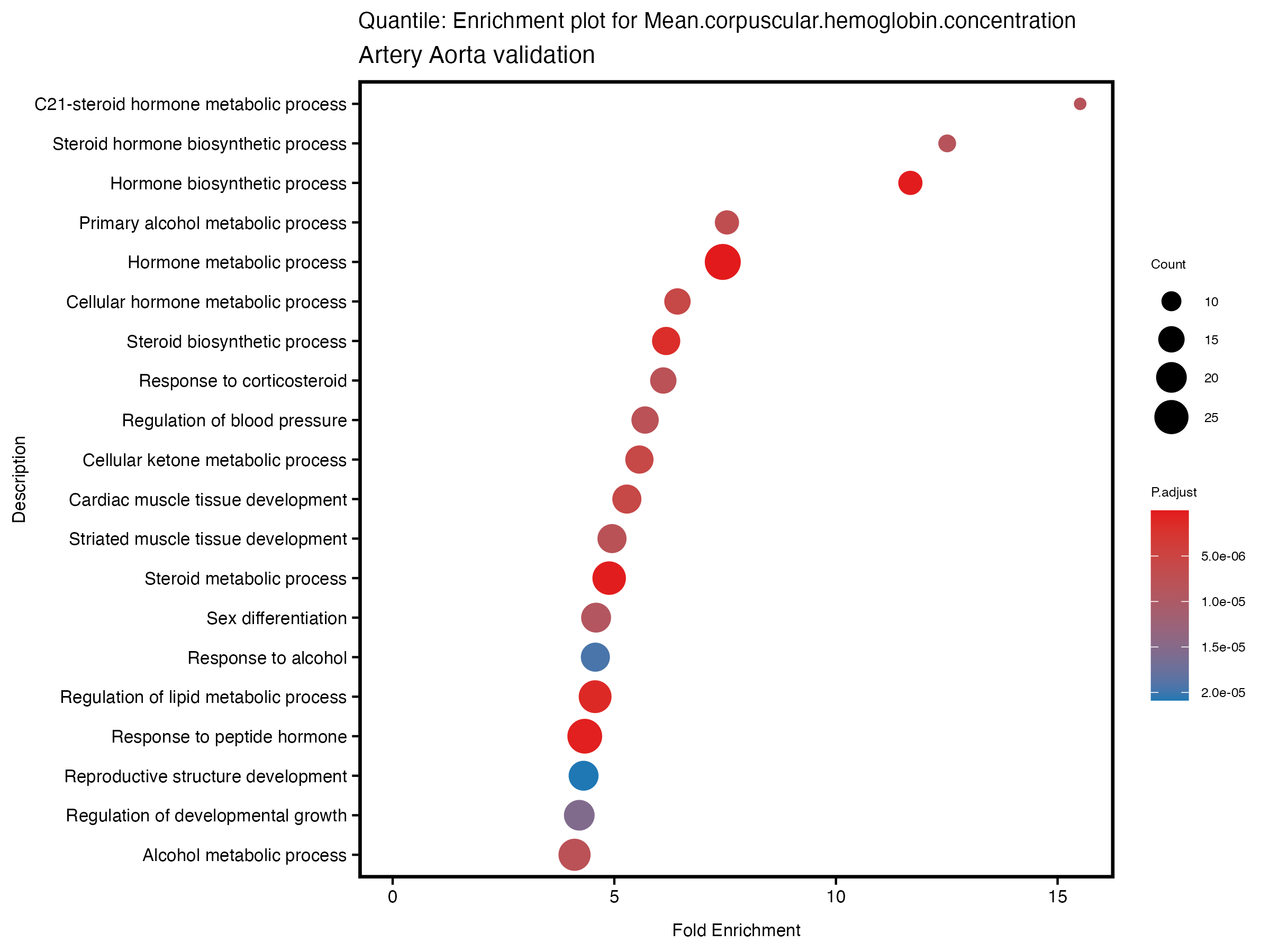
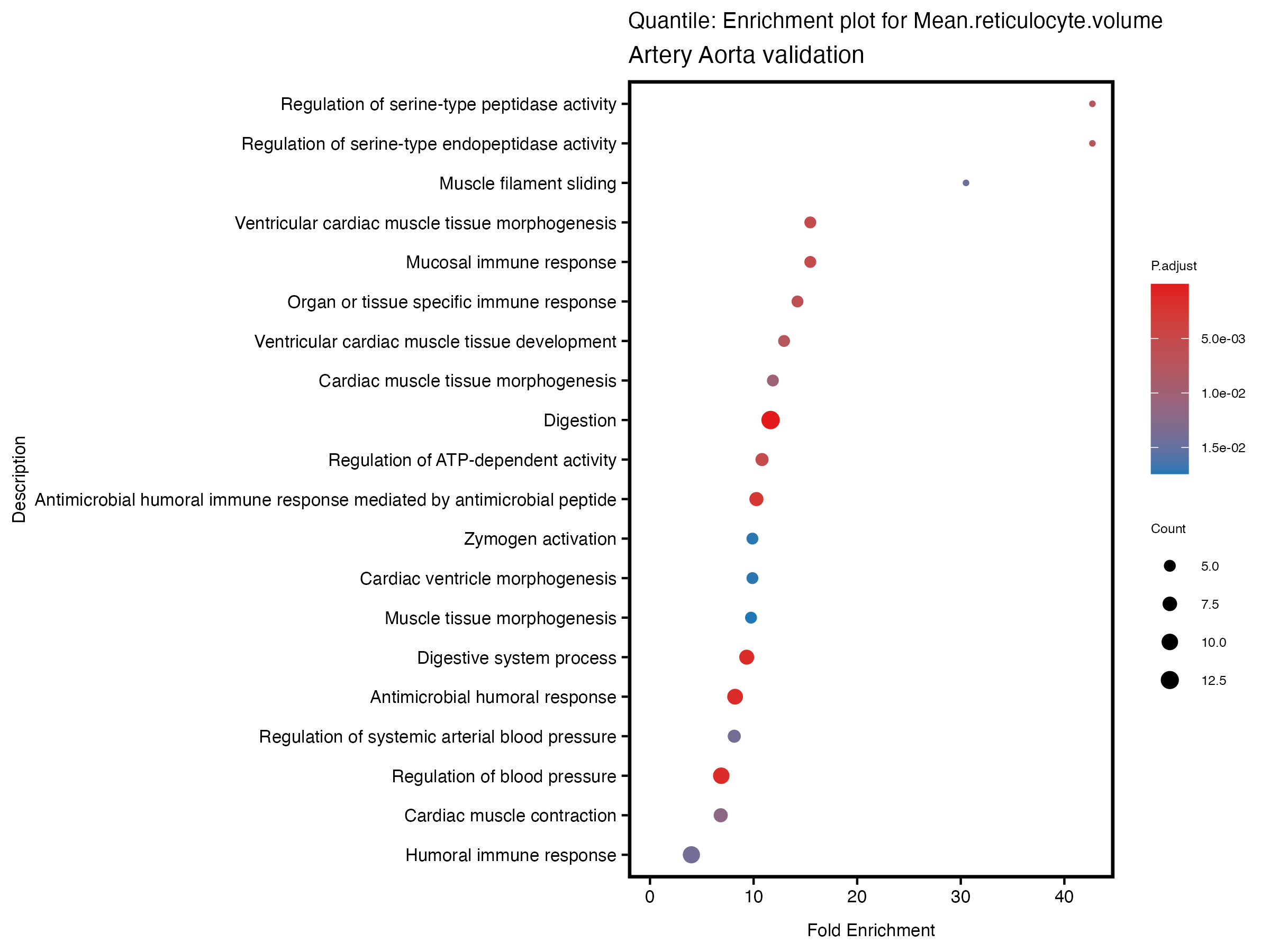
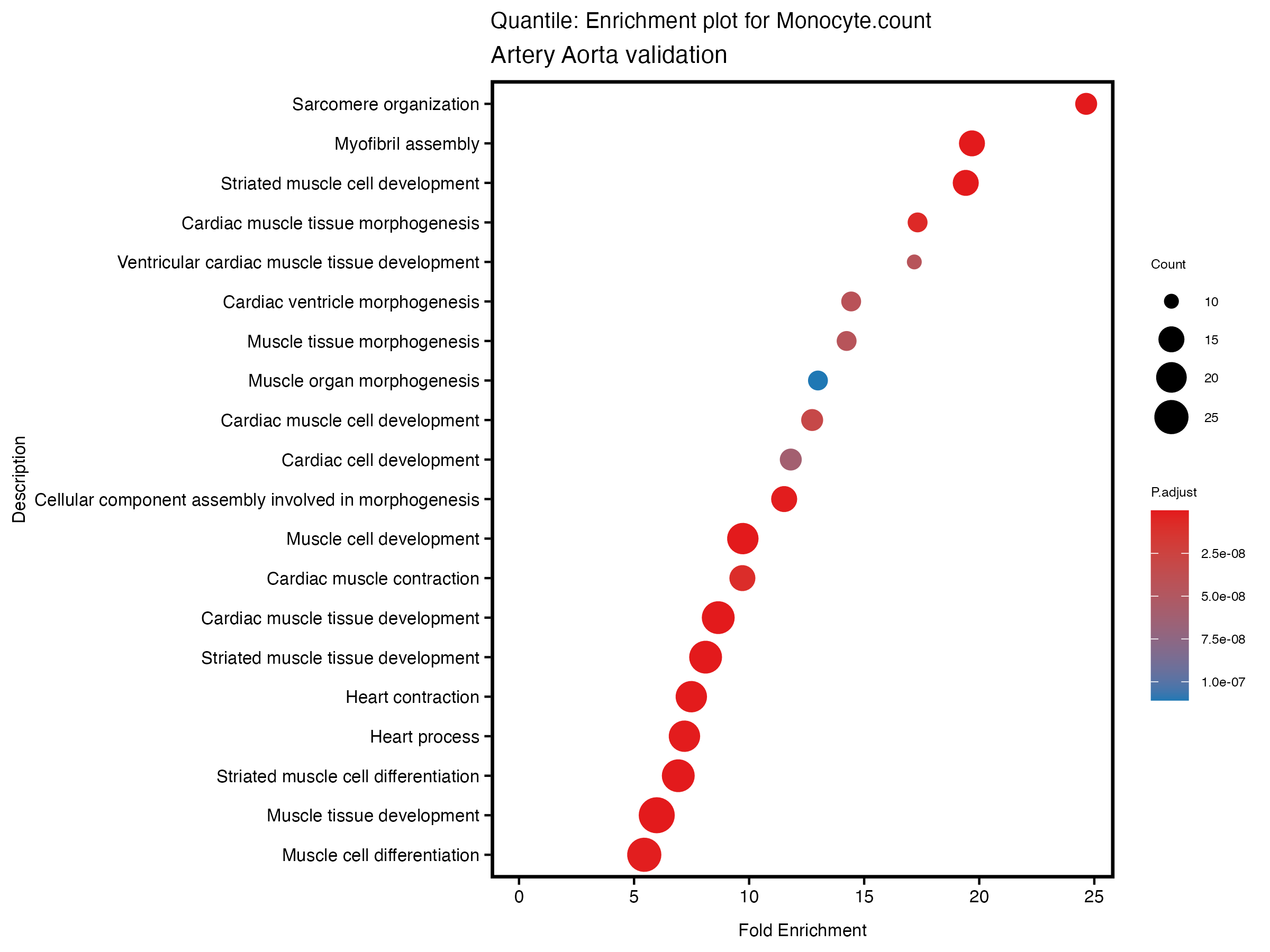
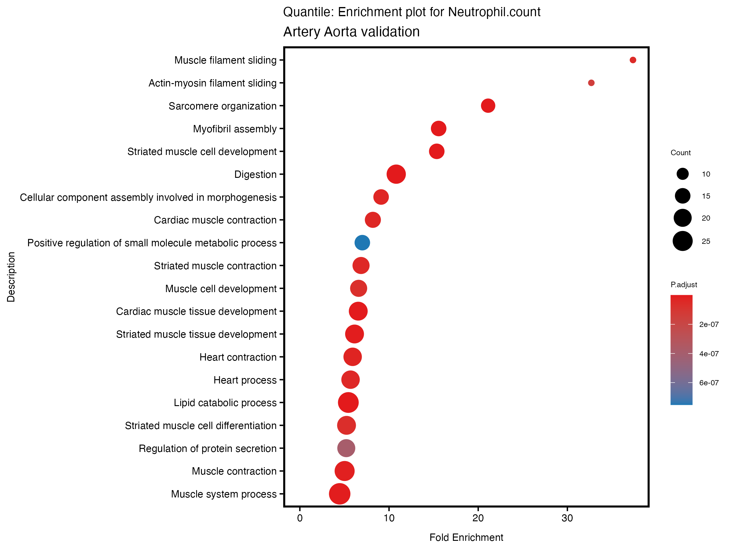
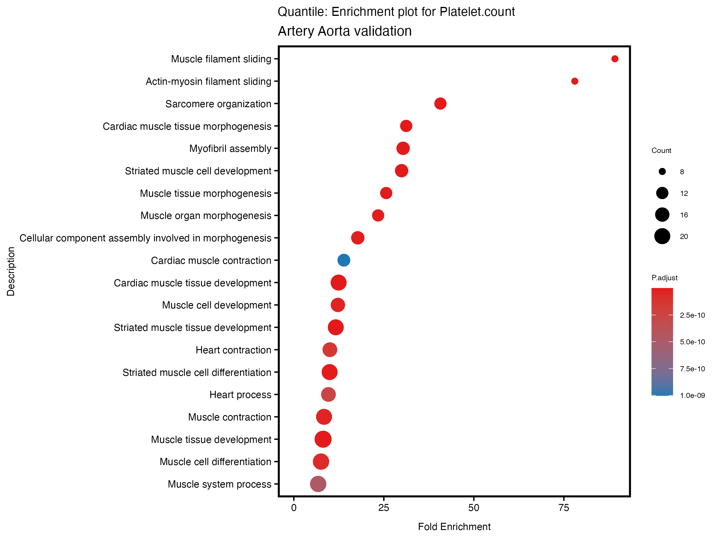
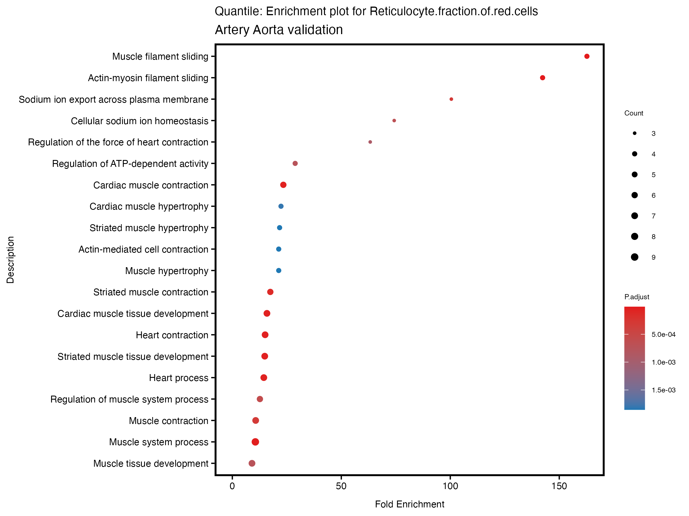
  gse <- enrichGO(gene = deGenes$gene_id, ont = "BP", 
                OrgDb ="org.Hs.eg.db", keyType = "ENSEMBL")
  
  write.csv(as.data.frame(gse), file = paste0("GO_enrichment_quantile_", trait, "_results_artery_validation.csv"))
  
  gse <- as.data.frame(gse)
  gse$GeneRatio_num <- as.numeric(sapply(strsplit(gse$GeneRatio, "/"), 
                                         function(x) x[1])) /
                     as.numeric(sapply(strsplit(gse$GeneRatio, "/"), function(x) x[2]))

  gse$BgRatio_num <- as.numeric(sapply(strsplit(gse$BgRatio, "/"), function(x) x[1])) / 
                     as.numeric(sapply(strsplit(gse$BgRatio, "/"), function(x) x[2]))
  
  gse <- cbind(gse, FoldEnrich = gse$GeneRatio_num/gse$BgRatio_num)
  
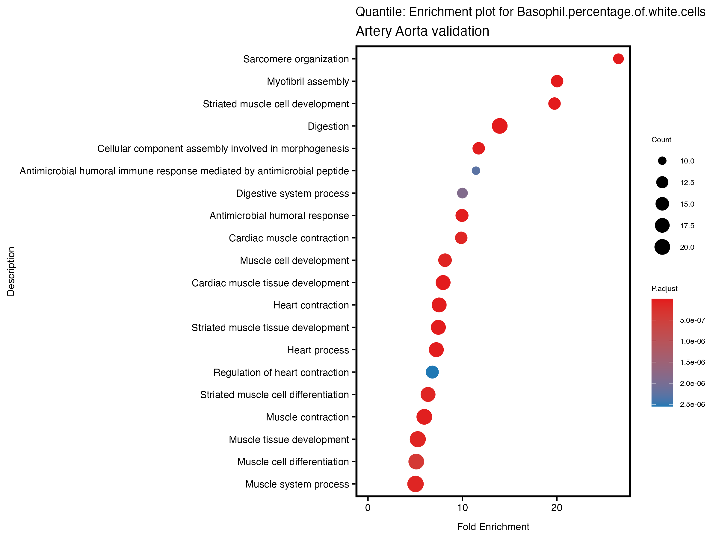
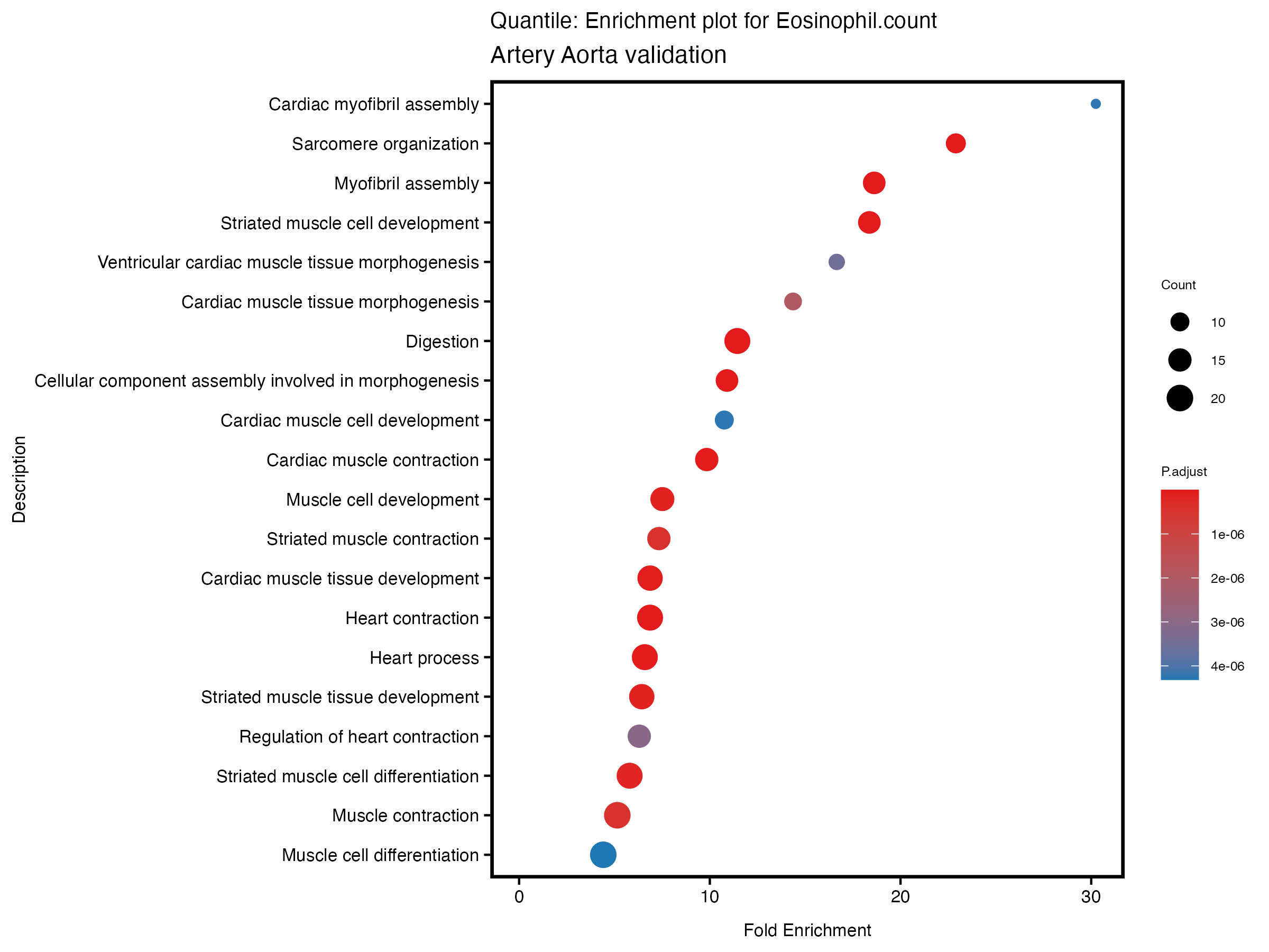
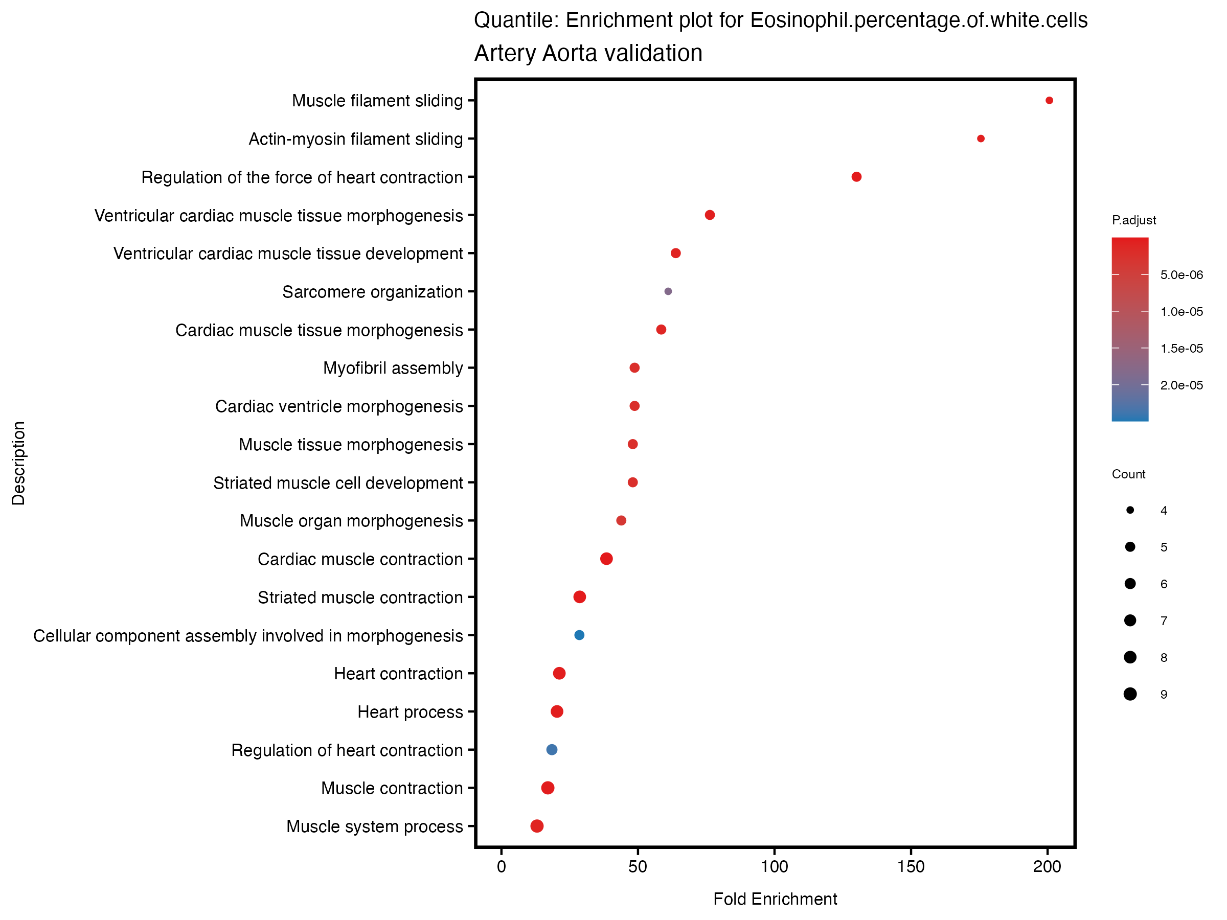
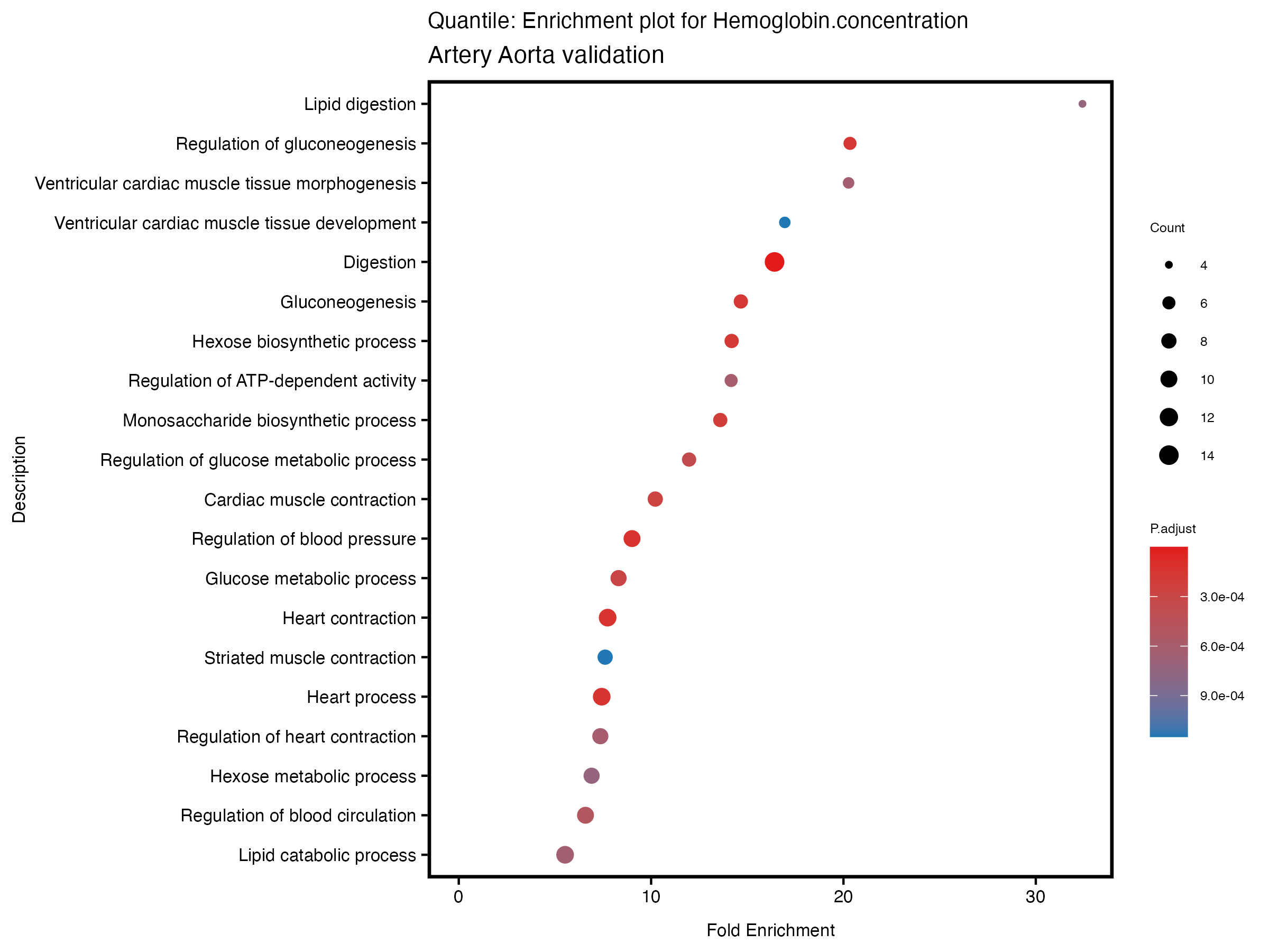
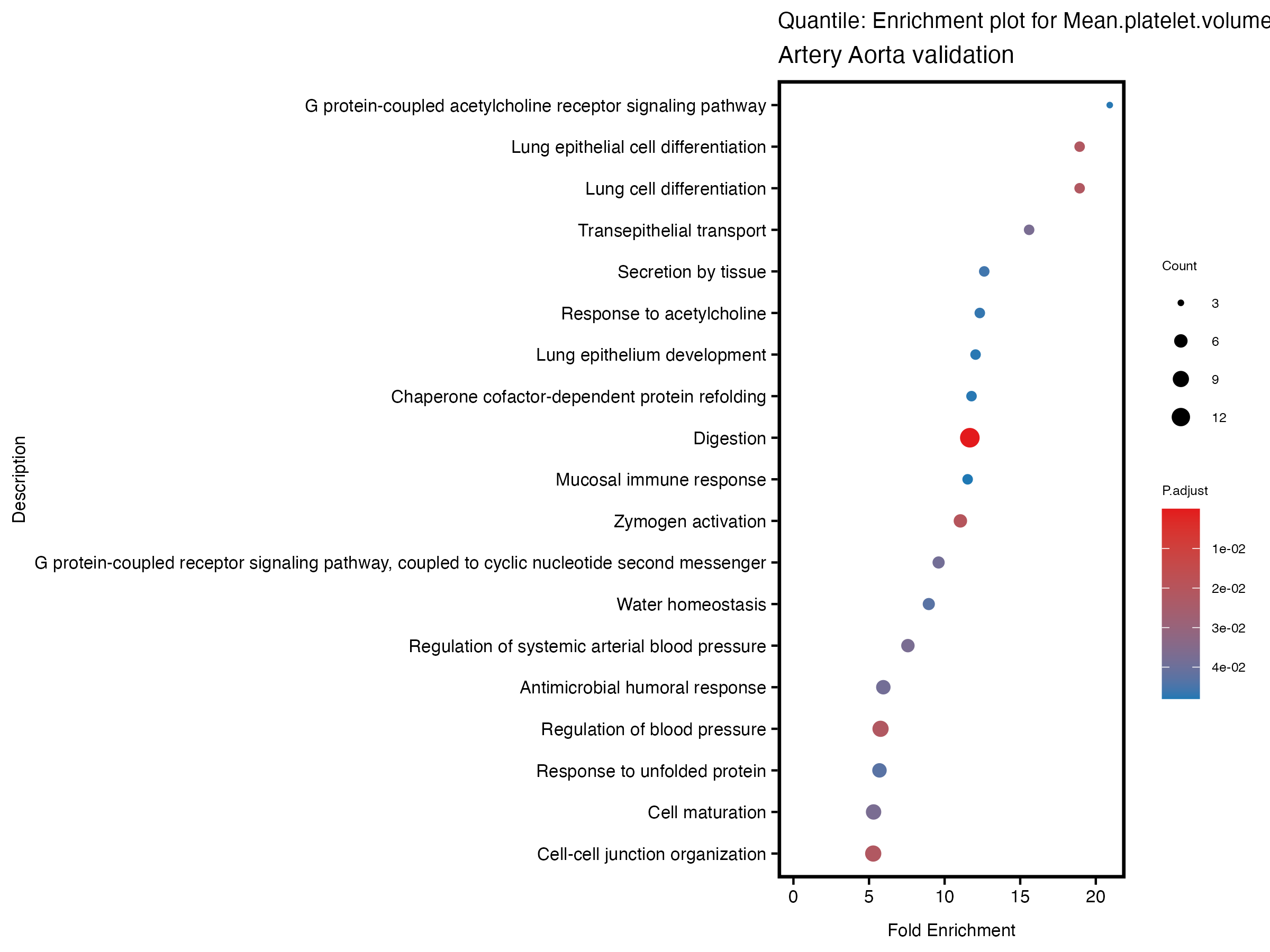
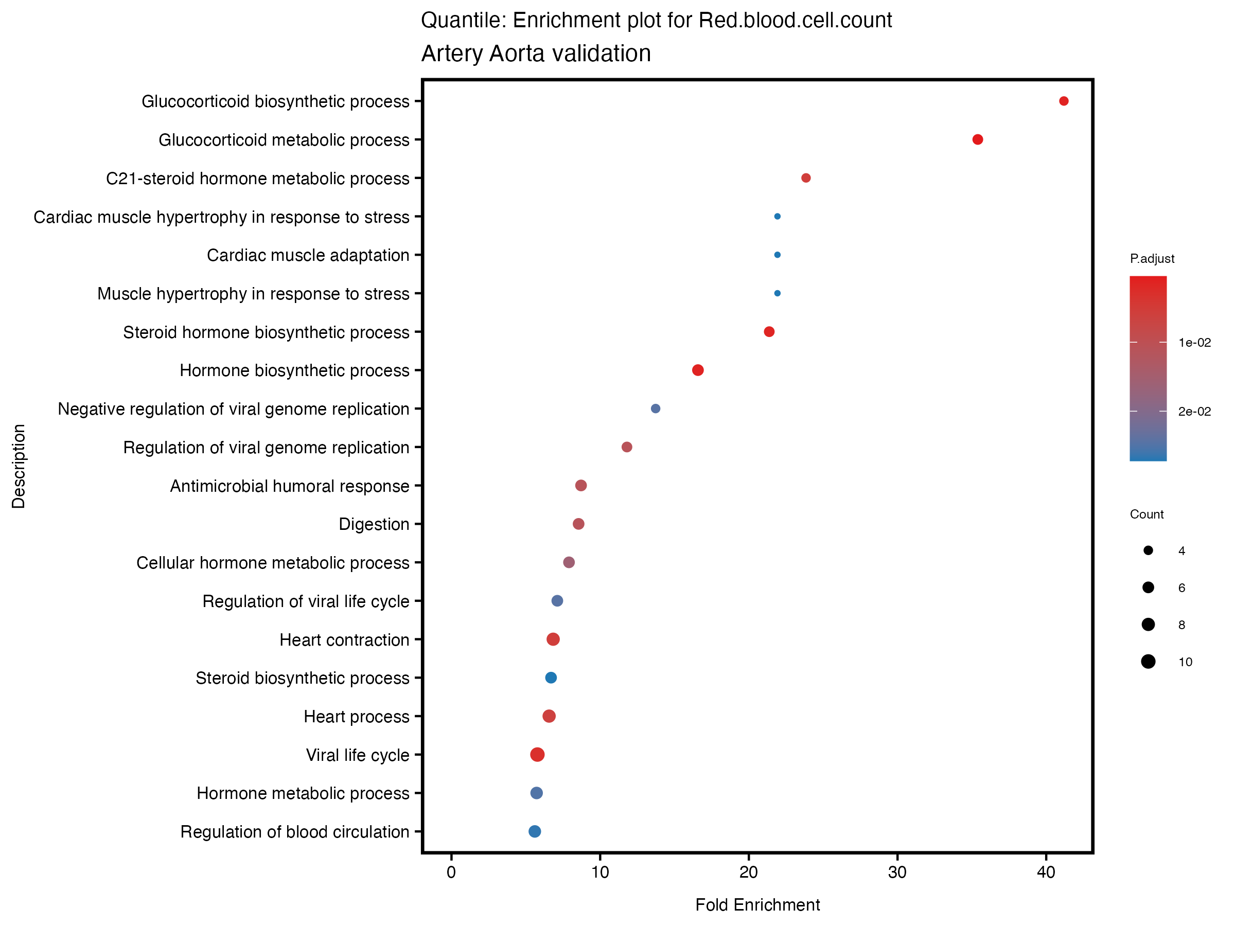
  if (nrow(gse) >= 20) {
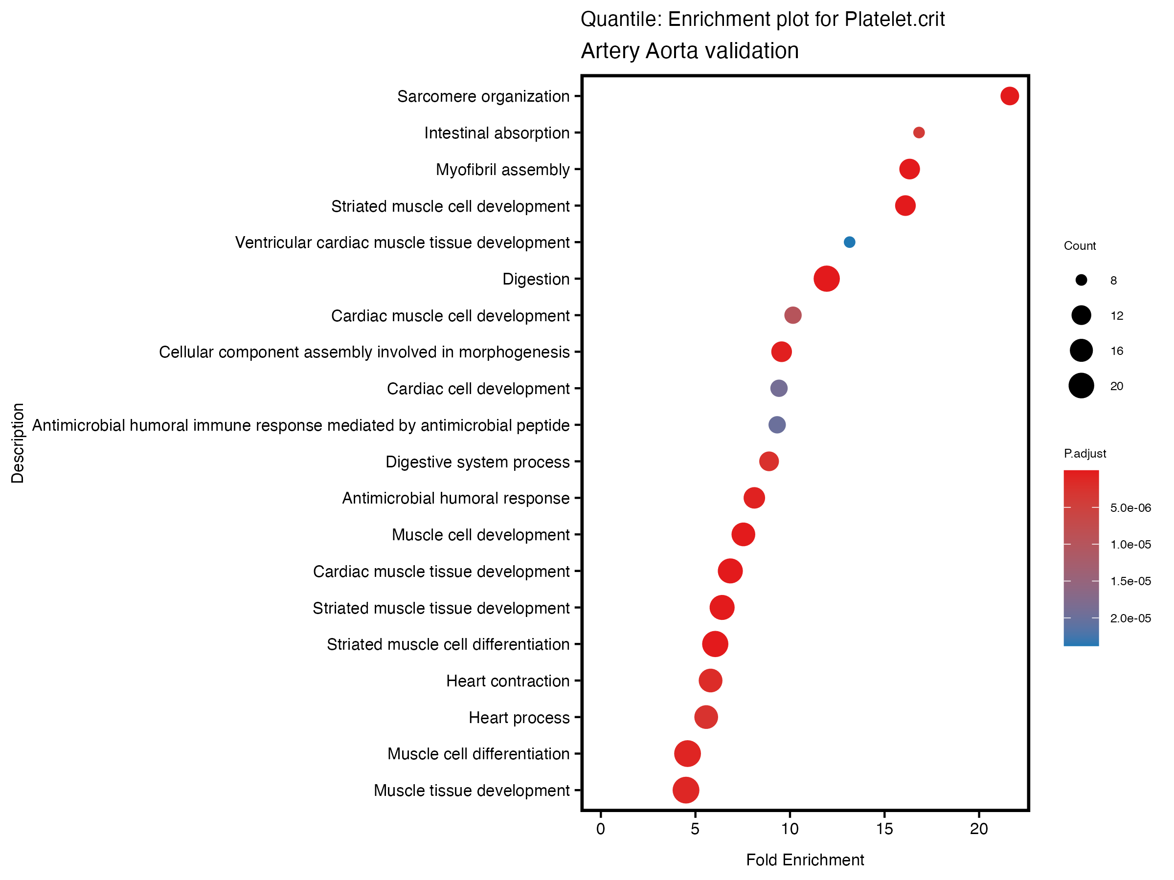
    enrich_plot <- plotEnrich(gse[1:20,], plot_type = "dot", scale_ratio = 0.5) +
    labs(title = paste("Quantile: Enrichment plot for", trait), 
         subtitle = "Artery Aorta validation") + 
    theme(plot.title = element_text(size = 10)) 
  }else{
    enrich_plot <- plotEnrich(gse, plot_type = "dot", scale_ratio = 0.5) +
    labs(title = paste("Quantile: Enrichment plot for", trait), 
         subtitle = "Artery Aorta validation") + 
    theme(plot.title = element_text(size = 10)) 
  }
  ggsave(paste0("enrichment_plot_quantile_", trait, "_artery_validation.png"), plot = enrich_plot, width = 8, height = 6)
}

Result

continuous_dir <- "analysis/continuous_artery"
quantile_dir <- "analysis/quantile_artery"

# Get the list of differential expression results and GO enrichment results
de_files_continuous <- list.files(continuous_dir, pattern = "differential_expression_.*_results_artery_validation.csv", 
                                  full.names = TRUE)
go_files_continuous <- list.files(continuous_dir, pattern = "GO_enrichment_.*_results_artery_validation.csv", 
                                  full.names = TRUE)

de_files_quantile <- list.files(quantile_dir, pattern = "differential_expression_.*_quantile_results_artery_validation.csv", 
                                full.names = TRUE)
go_files_quantile <- list.files(quantile_dir, pattern = "GO_enrichment_quantile_.*_results_artery_validation.csv", 
                                full.names = TRUE)

# Initialize a data frame to store the results
results_df_continuous <- data.frame(trait = character(),
                                    num_significant_de = integer(),
                                    upregulated = integer(),
                                    downregulated = integer(),
                                    num_enriched_go = integer(),
                                    stringsAsFactors = FALSE)

results_df_quantile <- data.frame(trait = character(),
                                  num_significant_de = integer(),
                                  upregulated = integer(),
                                  downregulated = integer(),
                                  num_enriched_go = integer(),
                                  stringsAsFactors = FALSE)

# Function to extract significant DE genes and GO enriched pathways
extract_results <- function(de_file, go_file, analysis_type) {
  # Load the differential expression results
  res <- read.csv(de_file, header = T, row.names = 1)
  
  # Filter for significant DE genes (padj < 0.1)
  significant_de <- res[!is.na(res$padj) & res$padj < 0.1, ]
  
  # Count number of upregulated and downregulated genes
  upregulated <- sum(significant_de$log2FoldChange > 0)
  downregulated <- sum(significant_de$log2FoldChange < 0)
  
  # Load the GO enrichment results
  go_res <- read.csv(go_file, header = T, row.names = 1)
  
  # Count the number of enriched GO pathways (adjusted p-value < 0.05)
  enriched_go <- sum(go_res$p.adjust < 0.05)
  
  if (analysis_type == "continuous"){
    # Extract trait name from the file name
    trait_name <- gsub("differential_expression_|_results.csv", "", basename(de_file))
    
    # Create a row for this trait and add it to the results data frame
    results_df_continuous <<- rbind(results_df_continuous, 
                                    data.frame(trait = trait_name,
                                               num_significant_de = nrow(significant_de),
                                               upregulated = upregulated,
                                              downregulated = downregulated,
                                              num_enriched_go = enriched_go))
  }else if (analysis_type == "quantile") {
    # Extract trait name from the file name
    trait_name <- gsub("differential_expression_|_quantile_results.csv", "", basename(de_file))
    
    # Create a row for this trait and add it to the results data frame
    results_df_quantile <<- rbind(
      results_df_quantile,
      data.frame(
        trait = trait_name,
        num_significant_de = nrow(significant_de),
        upregulated = upregulated,
        downregulated = downregulated,
        num_enriched_go = enriched_go
      )
    )
  }
}

# Loop through the continuous files and extract results
for (i in seq_along(de_files_continuous)) {
  extract_results(de_files_continuous[i], go_files_continuous[i], "continuous")
}

# Loop through the quantile files and extract results
for (i in seq_along(de_files_quantile)) {
  extract_results(de_files_quantile[i], go_files_quantile[i], "quantile")
}

colnames(results_df_continuous) <- c("Trait",
                          "Significant differential expressed genes", 
                          "Up", "Down", "Significant GO enriched pathways")
colnames(results_df_quantile) <- c("Trait",
                          "Significant differential expressed genes", 
                          "Up", "Down", "Significant GO enriched pathways")
knitr::kable(results_df_continuous, caption = "Continuous")

Continuous

Trait	Significant differential expressed genes	Up	Down	Significant GO enriched pathways
Basophil.count_results_artery_validation.csv	284	254	30	141
Basophil.percentage.of.white.cells_results_artery_validation.csv	349	273	76	109
Celiac_GCST90014442_results_artery_validation.csv	418	346	72	171
Celiac_GCST90468120_results_artery_validation.csv	103	16	87	111
Eosinophil.count_results_artery_validation.csv	251	186	65	121
Eosinophil.percentage.of.white.cells_results_artery_validation.csv	139	12	127	69
Hematocrit_results_artery_validation.csv	184	38	146	78
Hemoglobin.concentration_results_artery_validation.csv	217	77	140	88
High.light.scatter.reticulocyte.count_results_artery_validation.csv	67	56	11	2
High.light.scatter.reticulocyte.percentage.of.red.cells_results_artery_validation.csv	93	80	13	22
IBD_GCST90013901_results_artery_validation.csv	373	107	266	149
IBD_GCST90013951_results_artery_validation.csv	479	135	344	151
Immature.fraction.of.reticulocytes_results_artery_validation.csv	269	159	110	101
LUPUS_GCST003156_results_artery_validation.csv	132	44	88	7
LUPUS_GCST011096_results_artery_validation.csv	131	52	79	32
Lymphocyte.count_results_artery_validation.csv	197	89	108	55
Lymphocyte.percentage.of.white.cells_results_artery_validation.csv	200	17	183	116
Mean.corpuscular.hemoglobin_results_artery_validation.csv	293	103	190	77
Mean.corpuscular.hemoglobin.concentration_results_artery_validation.csv	1057	172	885	144
Mean.corpuscular.volume_results_artery_validation.csv	205	140	65	77
Mean.platelet.volume_results_artery_validation.csv	155	126	29	63
Mean.reticulocyte.volume_results_artery_validation.csv	115	77	38	76
Mean.sphered.corpuscular.volume_results_artery_validation.csv	73	29	44	38
Monocyte.count_results_artery_validation.csv	206	185	21	130
Monocyte.percentage.of.white.cells_results_artery_validation.csv	77	53	24	19
Neutrophil.count_results_artery_validation.csv	436	307	129	183
Neutrophil.percentage.of.white.cells_results_artery_validation.csv	466	313	153	220
Platelet.count_results_artery_validation.csv	139	68	71	137
Platelet.crit_results_artery_validation.csv	310	169	141	229
Platelet.distribution.width_results_artery_validation.csv	251	180	71	73
Red.blood.cell.count_results_artery_validation.csv	162	25	137	65
Red.cell.distribution.width_results_artery_validation.csv	242	93	149	74
Reticulocyte.count_results_artery_validation.csv	33	18	15	42
Reticulocyte.fraction.of.red.cells_results_artery_validation.csv	47	33	14	52
T1D_GCST90000529_results_artery_validation.csv	123	100	23	74
T1D_GCST90014023_results_artery_validation.csv	447	282	165	140
White.blood.cell.count_results_artery_validation.csv	481	412	69	183

knitr::kable(results_df_quantile, caption = "Quantile (Stratify trait into top 25% and remaining)")

Quantile (Stratify trait into top 25% and remaining)

Trait	Significant differential expressed genes	Up	Down	Significant GO enriched pathways
Basophil.count_quantile_results_artery_validation.csv	325	292	33	135
Basophil.percentage.of.white.cells_quantile_results_artery_validation.csv	218	186	32	125
Celiac_GCST90014442_quantile_results_artery_validation.csv	392	332	60	135
Celiac_GCST90468120_quantile_results_artery_validation.csv	72	26	46	103
Eosinophil.count_quantile_results_artery_validation.csv	249	209	40	133
Eosinophil.percentage.of.white.cells_quantile_results_artery_validation.csv	32	6	26	64
Hematocrit_quantile_results_artery_validation.csv	127	63	64	159
Hemoglobin.concentration_quantile_results_artery_validation.csv	122	84	38	153
High.light.scatter.reticulocyte.count_quantile_results_artery_validation.csv	60	17	43	134
High.light.scatter.reticulocyte.percentage.of.red.cells_quantile_results_artery_validation.csv	134	105	29	55
IBD_GCST90013901_quantile_results_artery_validation.csv	159	115	44	139
IBD_GCST90013951_quantile_results_artery_validation.csv	226	108	118	139
Immature.fraction.of.reticulocytes_quantile_results_artery_validation.csv	140	101	39	111
LUPUS_GCST003156_quantile_results_artery_validation.csv	143	57	86	78
LUPUS_GCST011096_quantile_results_artery_validation.csv	163	68	95	114
Lymphocyte.count_quantile_results_artery_validation.csv	278	100	178	89
Lymphocyte.percentage.of.white.cells_quantile_results_artery_validation.csv	127	22	105	123
Mean.corpuscular.hemoglobin_quantile_results_artery_validation.csv	319	143	176	119
Mean.corpuscular.hemoglobin.concentration_quantile_results_artery_validation.csv	793	133	660	471
Mean.corpuscular.volume_quantile_results_artery_validation.csv	269	166	103	144
Mean.platelet.volume_quantile_results_artery_validation.csv	193	164	29	19
Mean.reticulocyte.volume_quantile_results_artery_validation.csv	167	49	118	48
Mean.sphered.corpuscular.volume_quantile_results_artery_validation.csv	188	21	167	86
Monocyte.count_quantile_results_artery_validation.csv	575	359	216	108
Monocyte.percentage.of.white.cells_quantile_results_artery_validation.csv	169	109	60	145
Neutrophil.count_quantile_results_artery_validation.csv	339	247	92	363
Neutrophil.percentage.of.white.cells_quantile_results_artery_validation.csv	551	373	178	268
Platelet.count_quantile_results_artery_validation.csv	152	129	23	124
Platelet.crit_quantile_results_artery_validation.csv	310	275	35	153
Platelet.distribution.width_quantile_results_artery_validation.csv	354	309	45	181
Red.blood.cell.count_quantile_results_artery_validation.csv	118	26	92	29
Red.cell.distribution.width_quantile_results_artery_validation.csv	172	75	97	150
Reticulocyte.count_quantile_results_artery_validation.csv	61	26	35	99
Reticulocyte.fraction.of.red.cells_quantile_results_artery_validation.csv	39	15	24	73
T1D_GCST90000529_quantile_results_artery_validation.csv	131	95	36	45
T1D_GCST90014023_quantile_results_artery_validation.csv	379	266	113	170
White.blood.cell.count_quantile_results_artery_validation.csv	284	231	53	260

Session information

sessionInfo()

R version 4.2.2 (2022-10-31)
Platform: x86_64-apple-darwin17.0 (64-bit)
Running under: macOS Big Sur ... 10.16

Matrix products: default
BLAS:   /Library/Frameworks/R.framework/Versions/4.2/Resources/lib/libRblas.0.dylib
LAPACK: /Library/Frameworks/R.framework/Versions/4.2/Resources/lib/libRlapack.dylib

locale:
[1] en_US.UTF-8/en_US.UTF-8/en_US.UTF-8/C/en_US.UTF-8/en_US.UTF-8

attached base packages:
[1] stats4    stats     graphics  grDevices utils     datasets  methods  
[8] base     

other attached packages:
 [1] clusterProfiler_4.6.2       enrichplot_1.18.4          
 [3] org.Hs.eg.db_3.16.0         AnnotationDbi_1.60.2       
 [5] genekitr_1.2.8              ggrepel_0.9.6              
 [7] BiocParallel_1.32.6         DESeq2_1.38.3              
 [9] SummarizedExperiment_1.28.0 Biobase_2.58.0             
[11] MatrixGenerics_1.10.0       matrixStats_1.2.0          
[13] GenomicRanges_1.50.2        GenomeInfoDb_1.34.9        
[15] IRanges_2.32.0              S4Vectors_0.36.2           
[17] BiocGenerics_0.44.0         corrplot_0.95              
[19] ggplot2_3.5.1               dplyr_1.1.4                
[21] data.table_1.16.4           workflowr_1.7.1            

loaded via a namespace (and not attached):
  [1] shadowtext_0.1.4       fastmatch_1.1-6        plyr_1.8.9            
  [4] igraph_1.5.1           lazyeval_0.2.2         splines_4.2.2         
  [7] usethis_3.1.0          urltools_1.7.3         digest_0.6.37         
 [10] yulab.utils_0.2.0      htmltools_0.5.8.1      GOSemSim_2.24.0       
 [13] viridis_0.6.5          GO.db_3.16.0           magrittr_2.0.3        
 [16] memoise_2.0.1          remotes_2.5.0          openxlsx_4.2.5.2      
 [19] Biostrings_2.66.0      annotate_1.76.0        graphlayouts_1.0.1    
 [22] prettyunits_1.2.0      colorspace_2.1-1       blob_1.2.4            
 [25] xfun_0.50              callr_3.7.6            crayon_1.5.3          
 [28] RCurl_1.98-1.16        jsonlite_1.8.9         scatterpie_0.2.4      
 [31] ape_5.7-1              glue_1.8.0             polyclip_1.10-7       
 [34] gtable_0.3.6           zlibbioc_1.44.0        XVector_0.38.0        
 [37] DelayedArray_0.24.0    pkgbuild_1.4.6         scales_1.3.0          
 [40] DOSE_3.24.2            DBI_1.2.3              miniUI_0.1.1.1        
 [43] Rcpp_1.0.14            viridisLite_0.4.2      xtable_1.8-4          
 [46] progress_1.2.3         gridGraphics_0.5-1     tidytree_0.4.6        
 [49] bit_4.5.0.1            europepmc_0.4.3        profvis_0.4.0         
 [52] htmlwidgets_1.6.4      httr_1.4.7             fgsea_1.24.0          
 [55] RColorBrewer_1.1-3     ellipsis_0.3.2         urlchecker_1.0.1      
 [58] pkgconfig_2.0.3        XML_3.99-0.18          farver_2.1.2          
 [61] sass_0.4.9             locfit_1.5-9.8         ggplotify_0.1.2       
 [64] tidyselect_1.2.1       rlang_1.1.5            reshape2_1.4.4        
 [67] later_1.4.1            munsell_0.5.1          tools_4.2.2           
 [70] cachem_1.1.0           downloader_0.4         cli_3.6.3             
 [73] generics_0.1.3         RSQLite_2.3.9          gson_0.1.0            
 [76] devtools_2.4.5         evaluate_1.0.3         stringr_1.5.1         
 [79] fastmap_1.2.0          yaml_2.3.10            ggtree_3.6.2          
 [82] processx_3.8.5         knitr_1.49             bit64_4.6.0-1         
 [85] fs_1.6.5               tidygraph_1.3.0        zip_2.3.2             
 [88] purrr_1.0.2            KEGGREST_1.38.0        ggraph_2.1.0          
 [91] nlme_3.1-160           mime_0.12              whisker_0.4.1         
 [94] aplot_0.2.4            ggvenn_0.1.10          xml2_1.3.6            
 [97] compiler_4.2.2         rstudioapi_0.17.1      png_0.1-8             
[100] treeio_1.22.0          tibble_3.2.1           tweenr_2.0.3          
[103] geneplotter_1.76.0     bslib_0.9.0            stringi_1.8.4         
[106] ps_1.8.1               lattice_0.22-6         Matrix_1.5-1          
[109] vctrs_0.6.5            pillar_1.10.1          lifecycle_1.0.4       
[112] triebeard_0.4.1        jquerylib_0.1.4        cowplot_1.1.3         
[115] bitops_1.0-9           httpuv_1.6.15          patchwork_1.3.0       
[118] qvalue_2.30.0          R6_2.5.1               promises_1.3.2        
[121] gridExtra_2.3          sessioninfo_1.2.2      codetools_0.2-20      
[124] pkgload_1.4.0          MASS_7.3-58.1          rprojroot_2.0.4       
[127] withr_3.0.2            GenomeInfoDbData_1.2.9 parallel_4.2.2        
[130] hms_1.1.3              grid_4.2.2             ggfun_0.1.8           
[133] tidyr_1.3.1            HDO.db_0.99.1          rmarkdown_2.29        
[136] git2r_0.33.0           getPass_0.2-4          ggforce_0.4.1         
[139] shiny_1.10.0           geneset_0.2.7